Vowel Normalization in R
- What is vowel normalization?
- Types of vowel normalization
- Which method is best?
I will be using the following packages in this workshop. If you do not have them installed now, please install them. I also will be using this colorblind-friendly palette for my plotting, when possible.
library(tidyverse)
library(phonR)
library(phonTools)
library(vowels)
cbPalette <- c("#999999", "#E69F00", "#56B4E9", "#009E73", "#F0E442", "#0072B2", "#D55E00", "#CC79A7")
What is vowel normalization?
Vowel normalization is, broadly speaking, a way to make acoustic data comparable across individual speakers. This is done by eliminating differences between acoustic outputs that arise due to different social and physical differences. Normalization is done in many different contexts, including (but not limited to!) cross-gender and/or cross-age comparisons, cross- and within-sociolinguistic community comparisons, longitudinal studies, etc.
There are three main types of information conveyed by a speaker to a listener (Ladefoged and Broadbent, 1957). All three of these types of information systematically affect formant frequencies in some way.
- Phonemic information
- anatomical/physiological information
- sociolinguistic information
There are four general goals listed for vowel normalization (based on Flynn and Foulkes, 2011; Watt et al., 2010). The type of normalization done depends on the goal of your research project.
- minimize inter-speaker variation due to physiological or anatomical differences
- preserve inter-speaker variation in vowel quality due to dialectal or social factors, or to preserve features in a sound change
- maintain phonological differences
- model cognitive processes that allow listeners to understand different speakers.
To demonstrate these types of normalization, I will use two datasets: 1) the Peterson and Barney (1952) vowel dataset, available through the phonTools package (There are 76 speakers, each producing 2 repetitions of 10 vowels, for a total of 1520 observations), and 2) the Indonesian vowels dataset, available through the phonR package (There are 8 speakers, five vowels, an uneven number of repetitions, for a total of 1725 observations).
library(phonTools)
data(pb52)
str(pb52)
## 'data.frame': 1520 obs. of 9 variables:
## $ type : Factor w/ 3 levels "c","m","w": 2 2 2 2 2 2 2 2 2 2 ...
## $ sex : Factor w/ 2 levels "f","m": 2 2 2 2 2 2 2 2 2 2 ...
## $ speaker : int 1 1 1 1 1 1 1 1 1 1 ...
## $ vowel : Factor w/ 10 levels "{","3'","A","E",..: 5 5 6 6 4 4 1 1 10 10 ...
## $ repetition: int 1 2 1 2 1 2 1 2 1 2 ...
## $ f0 : int 160 186 203 192 161 155 140 180 144 148 ...
## $ f1 : int 240 280 390 310 490 570 560 630 590 620 ...
## $ f2 : int 2280 2400 2030 1980 1870 1700 1820 1700 1250 1300 ...
## $ f3 : int 2850 2790 2640 2550 2420 2600 2660 2550 2620 2530 ...summary(pb52)## type sex speaker vowel repetition f0
## c:300 f:720 Min. : 1.00 { :152 Min. :1.0 Min. : 91.0
## m:660 m:800 1st Qu.:19.75 3' :152 1st Qu.:1.0 1st Qu.:133.0
## w:560 Median :38.50 A :152 Median :1.5 Median :200.0
## Mean :38.50 E :152 Mean :1.5 Mean :191.3
## 3rd Qu.:57.25 i :152 3rd Qu.:2.0 3rd Qu.:238.0
## Max. :76.00 I :152 Max. :2.0 Max. :350.0
## (Other):608
## f1 f2 f3
## Min. : 190.0 Min. : 560 Min. :1400
## 1st Qu.: 420.0 1st Qu.:1100 1st Qu.:2370
## Median : 540.0 Median :1470 Median :2680
## Mean : 563.3 Mean :1624 Mean :2708
## 3rd Qu.: 681.0 3rd Qu.:2100 3rd Qu.:3030
## Max. :1300.0 Max. :3610 Max. :4380
## pb52$speaker = as.factor(pb52$speaker)
pb52$vowelxsampa = pb52$vowel
levels(pb52$vowel)## [1] "{" "3'" "A" "E" "i" "I" "O" "u" "U" "V"levels(pb52$vowel) = c("æ", "ɚ", "ɑ", "ɛ", "i", "ɪ", "ɔ", "u", "ʊ","ʌ")
levels(pb52$vowel)## [1] "æ" "ɚ" "ɑ" "ɛ" "i" "ɪ" "ɔ" "u" "ʊ" "ʌ"head(pb52)## type sex speaker vowel repetition f0 f1 f2 f3 vowelxsampa
## 1 m m 1 i 1 160 240 2280 2850 i
## 2 m m 1 i 2 186 280 2400 2790 i
## 3 m m 1 ɪ 1 203 390 2030 2640 I
## 4 m m 1 ɪ 2 192 310 1980 2550 I
## 5 m m 1 ɛ 1 161 490 1870 2420 E
## 6 m m 1 ɛ 2 155 570 1700 2600 Elibrary(phonR)
data("indoVowels")
indo$subj = as.factor(indo$subj)
head(indo)## subj gender vowel f1 f2
## 1 F02 f a 1052 1800
## 2 F02 f a 904 1911
## 3 F02 f a 606 1829
## 4 F02 f a 652 1901
## 5 F02 f a 1129 1863
## 6 F02 f a 968 1699str(indo)## 'data.frame': 1725 obs. of 5 variables:
## $ subj : Factor w/ 8 levels "F02","F04","F08",..: 1 1 1 1 1 1 1 1 1 2 ...
## $ gender: Factor w/ 2 levels "f","m": 1 1 1 1 1 1 1 1 1 1 ...
## $ vowel : Factor w/ 5 levels "a","e","i","o",..: 1 1 1 1 1 1 1 1 1 1 ...
## $ f1 : int 1052 904 606 652 1129 968 1124 924 602 607 ...
## $ f2 : int 1800 1911 1829 1901 1863 1699 1882 1876 1815 1950 ...summary(indo)## subj gender vowel f1 f2
## F02 :225 f:867 a:349 Min. : 248.0 Min. : 489
## F04 :221 m:858 e:335 1st Qu.: 402.0 1st Qu.:1055
## M02 :219 i:348 Median : 493.0 Median :1509
## F08 :218 o:346 Mean : 531.1 Mean :1594
## M03 :217 u:347 3rd Qu.: 632.0 3rd Qu.:2097
## M04 :213 Max. :1129.0 Max. :3163
## (Other):412Types of vowel normalization
As mentioned above, there are different methods of doing vowel normalization, depending on the end goal of your study. We can classify these methods as having three traits: whether they are speaker-intrinsic or speaker-extrinsic, vowel-intrinsic or vowel-extrinsic, and formant-intrinsic or formant-extrinsic. Each of these refers to whether or not a calculation of normalization is being done on a single instance/measure of an object, or across multiple instances or measures.
Vowel: vowel intrinsic measures use only the acoustic information within a single vowel token to normalize said token, while vowel extrinsic measures use the acoustic information across more than one vowel of a talker (e.g., the “point” vowels or the whole vowel space of the speaker)
Formant: formant intrinsic measures use only a single formant for normalization, while formant extrinsic measures use multiple formants
Speaker: speaker intrinsic measures use only a single speaker’s data for normalization, while speaker extrinsic measures try to look at an entire population to modify the vowel space
I will go through different types of transformations used in the literature, and show you how they are implemented in R. First, I want to show you the vowel spaces without any transformation, so we can compare. Note that I will show you a lot of transformaiton methods available in the phonR and phontools packages. There is another package, called vowels, which also has functions for some of these transformations, but it requires data to be in a very particular structure, so I do not like to use it.
ggplot(pb52, aes(x = f2, y = f1, color = vowel)) + geom_point(aes(shape = vowel),alpha = 0.3) + stat_ellipse()+ theme_minimal() +scale_color_manual(values = cbPalette[c(1:8, 1, 2)]) + scale_x_reverse() + scale_y_reverse() + scale_shape_manual(values = 1:10)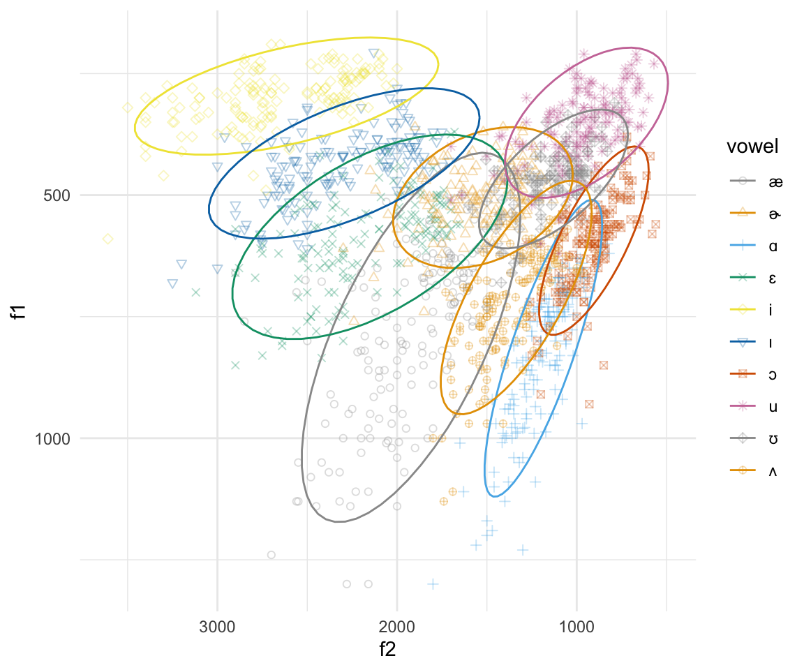
ggplot(pb52, aes(x = f2, y = f1, color = vowel)) + geom_point(aes(shape = vowel),alpha = 0.3) + stat_ellipse()+ theme_minimal() +scale_color_manual(values = c(cbPalette, cbPalette10)) + scale_shape_manual(values = 1:10)+ scale_x_reverse() + scale_y_reverse()  + geom_text(data=pb52 %>%
               group_by(vowel) %>%
               summarise_at(vars(f1:f2), mean, na.rm = TRUE), aes(label = vowel), size = 8)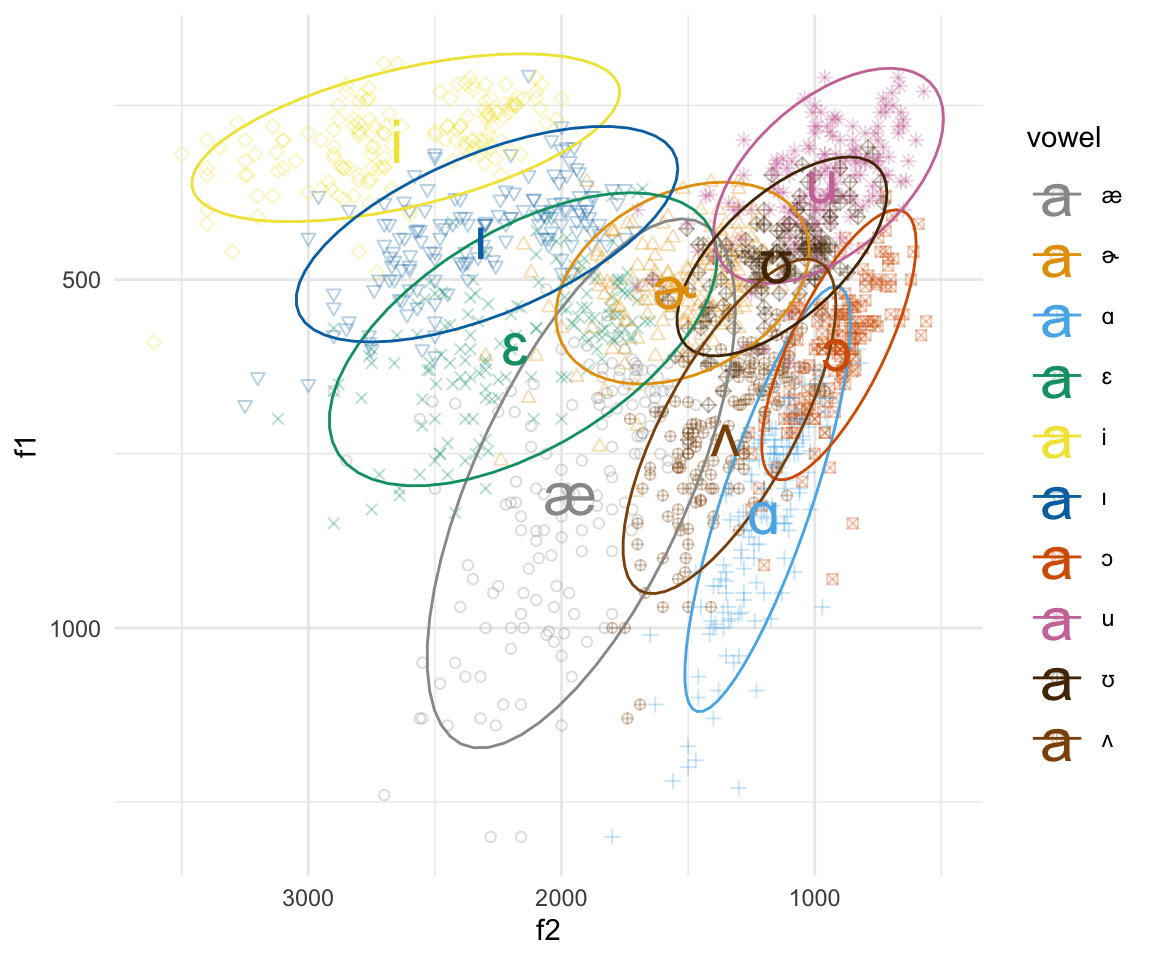
ggplot(pb52, aes(x = f2, y = f1, color = vowel))  + stat_ellipse()+ theme_minimal() +scale_color_manual(values = c(cbPalette, cbPalette10)) + scale_x_reverse() + scale_y_reverse()  + geom_text(data=pb52 %>%
               group_by(vowel) %>%
               summarise_at(vars(f1:f2), mean, na.rm = TRUE), aes(label = vowel), size = 8)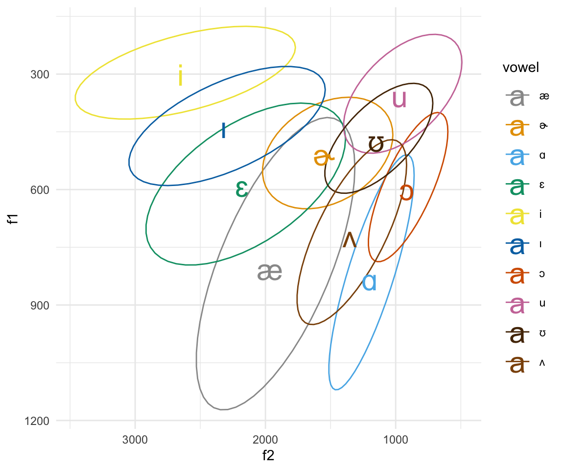
ggplot(indo, aes(x = f2, y = f1, color = vowel)) + geom_point(aes(shape = vowel),alpha = 0.3) + stat_ellipse()+ theme_minimal() +scale_color_manual(values = cbPalette) + scale_x_reverse() + scale_y_reverse() + scale_shape_manual(values = 1:10)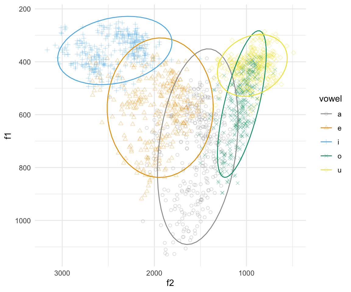
ggplot(indo, aes(x = f2, y = f1, color = vowel)) + geom_point(aes(shape = vowel),alpha = 0.3) + stat_ellipse()+ theme_minimal() +scale_color_manual(values = cbPalette) + scale_shape_manual(values = 1:10)+ scale_x_reverse() + scale_y_reverse()  + geom_text(data=indo %>%
               group_by(vowel) %>%
               summarise_at(vars(f1:f2), mean, na.rm = TRUE), aes(label = vowel), size = 8)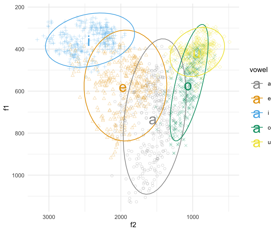
ggplot(indo, aes(x = f2, y = f1, color = vowel))  + stat_ellipse()+ theme_minimal() +scale_color_manual(values = c(cbPalette, cbPalette10)) + scale_x_reverse() + scale_y_reverse()  + geom_text(data=indo %>%
               group_by(subj,vowel) %>%
               summarise_at(vars(f1:f2), mean, na.rm = TRUE), aes(label = vowel), size = 6) + facet_wrap(~subj, ncol = 2)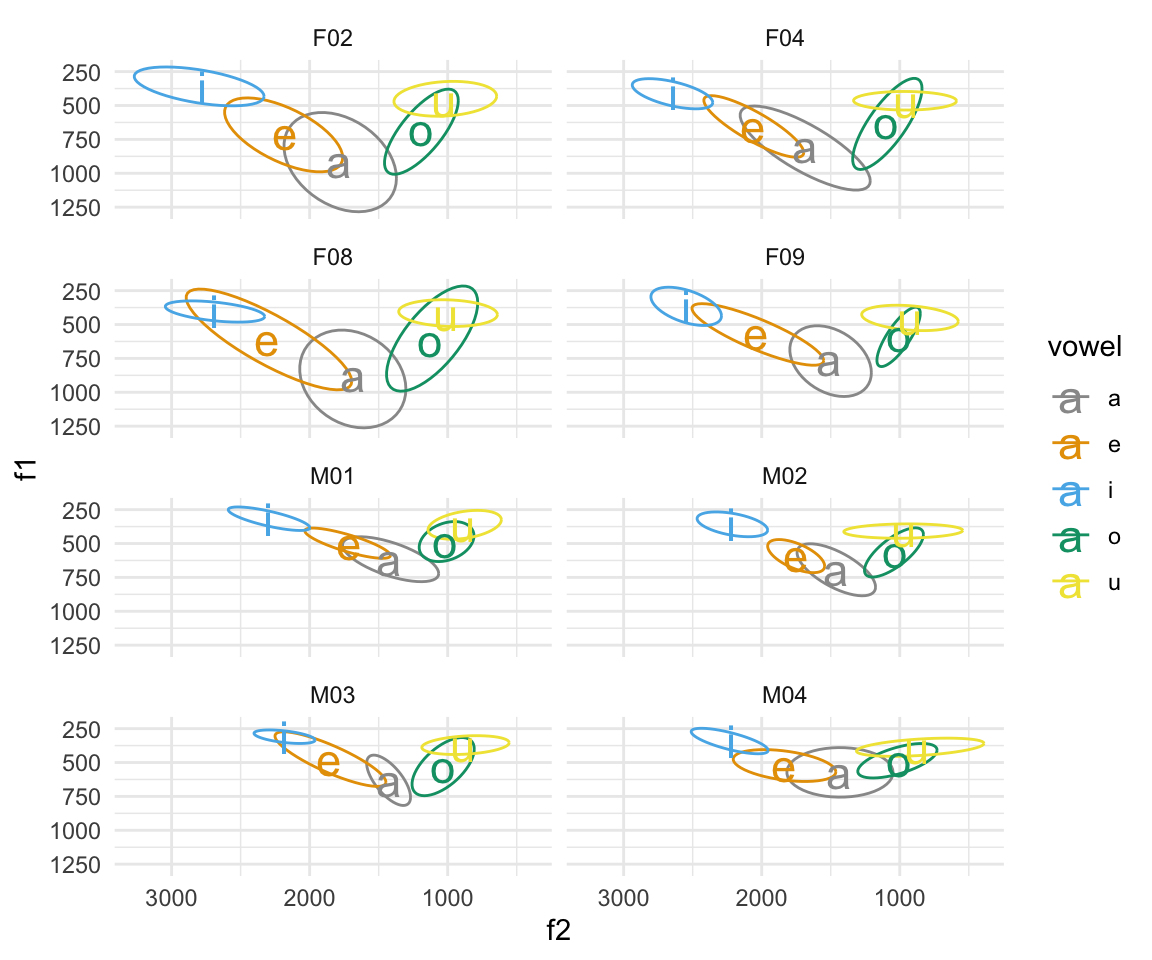
Speaker intrinsic/vowel intrinsic/formant intrinsic
Methods that are speaker, vowel, and formant intrinsic are often transformations that approximate the non-linear frequency response of the inner ear (hello basilar membrane!). That is, these transformations reflect the higher sensitivities to frequency changes in the lower end of the spectrum. There are a few psychoperceptual scales here, including log transformations, ERB transformation, mel transformation, and Bark transformation.
Log transformations
Log transformation is exactly what it sounds like: doing a logarithmic transformation of a value. Note that in R, the log() function does base-e (i.e., namtural logarithm) transformation. The log10() function performs base-10 logarithmic transformation.
pb52log = pb52 %>% mutate(f1log = log(f1), f2log = log(f2), f1log10 = log10(f1), f2log10 = log10(f2))
head(pb52log)
## type sex speaker vowel repetition f0 f1 f2 f3 vowelxsampa f1log
## 1 m m 1 i 1 160 240 2280 2850 i 5.480639
## 2 m m 1 i 2 186 280 2400 2790 i 5.634790
## 3 m m 1 ɪ 1 203 390 2030 2640 I 5.966147
## 4 m m 1 ɪ 2 192 310 1980 2550 I 5.736572
## 5 m m 1 ɛ 1 161 490 1870 2420 E 6.194405
## 6 m m 1 ɛ 2 155 570 1700 2600 E 6.345636
## f2log f1log10 f2log10
## 1 7.731931 2.380211 3.357935
## 2 7.783224 2.447158 3.380211
## 3 7.615791 2.591065 3.307496
## 4 7.590852 2.491362 3.296665
## 5 7.533694 2.690196 3.271842
## 6 7.438384 2.755875 3.230449ggplot(pb52log, aes(x = f2log, y = f1log, color = vowel)) + geom_point(aes(shape = vowel),alpha = 0.3) + stat_ellipse()+ theme_minimal() +scale_color_manual(values = cbPalette[c(1:8, 1, 2)]) + scale_x_reverse() + scale_y_reverse() + scale_shape_manual(values = 1:10)+ ggtitle("Log-transformed vowel plot (PB52 data)")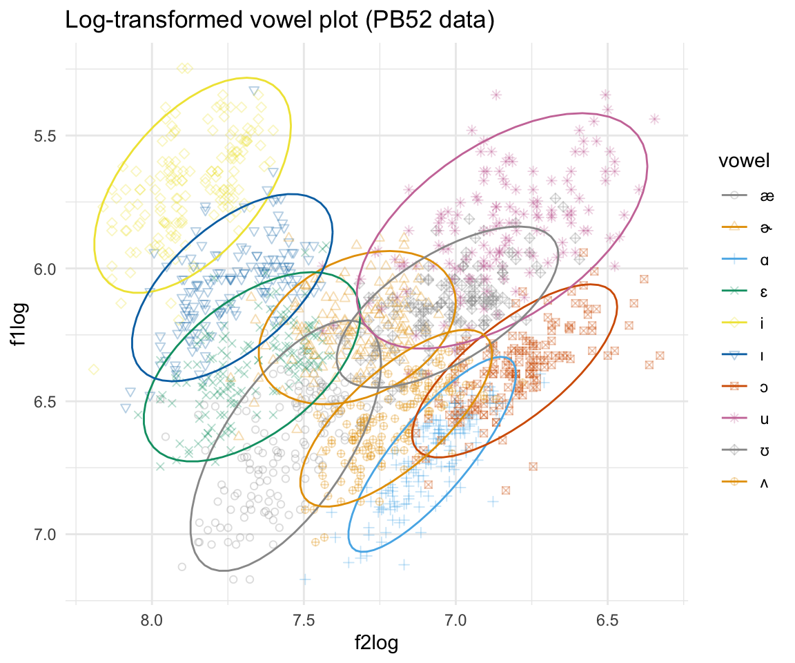
ggplot(pb52log, aes(x = f2log, y = f1log, color = vowel))  + stat_ellipse()+ theme_minimal() +scale_color_manual(values = c(cbPalette, cbPalette10)) + scale_x_reverse() + scale_y_reverse()  + geom_text(data=pb52log%>%group_by(vowel) %>%
               summarise_at(vars(f1log:f2log), mean, na.rm = TRUE), aes(label = vowel), size = 8)+ ggtitle("Log-transformed vowel plot (PB52 data)")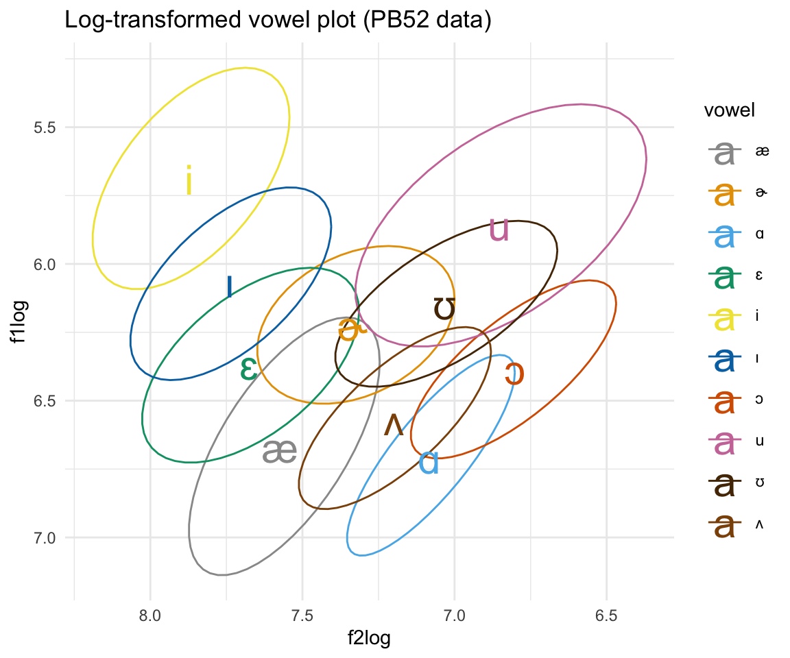
ggplot(pb52log, aes(x = f2log10, y = f1log10, color = vowel)) + geom_point(aes(shape = vowel),alpha = 0.3) + stat_ellipse()+ theme_minimal() +scale_color_manual(values = cbPalette[c(1:8, 1, 2)]) + scale_x_reverse() + scale_y_reverse() + scale_shape_manual(values = 1:10) + ggtitle("Log10-transformed vowel plot (PB52 data)")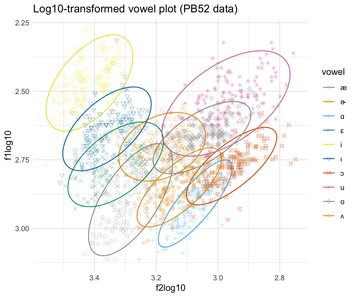
ggplot(pb52log, aes(x = f2log10,y = f1log10, color = vowel))  + stat_ellipse()+ theme_minimal() +scale_color_manual(values = c(cbPalette, cbPalette10)) + scale_x_reverse() + scale_y_reverse()  + geom_text(data=pb52log%>%group_by(vowel) %>%
               summarise_at(vars(f1log10:f2log10), mean, na.rm = TRUE), aes(label = vowel), size = 8)+ ggtitle("Log10-transformed vowel plot (PB52 data)")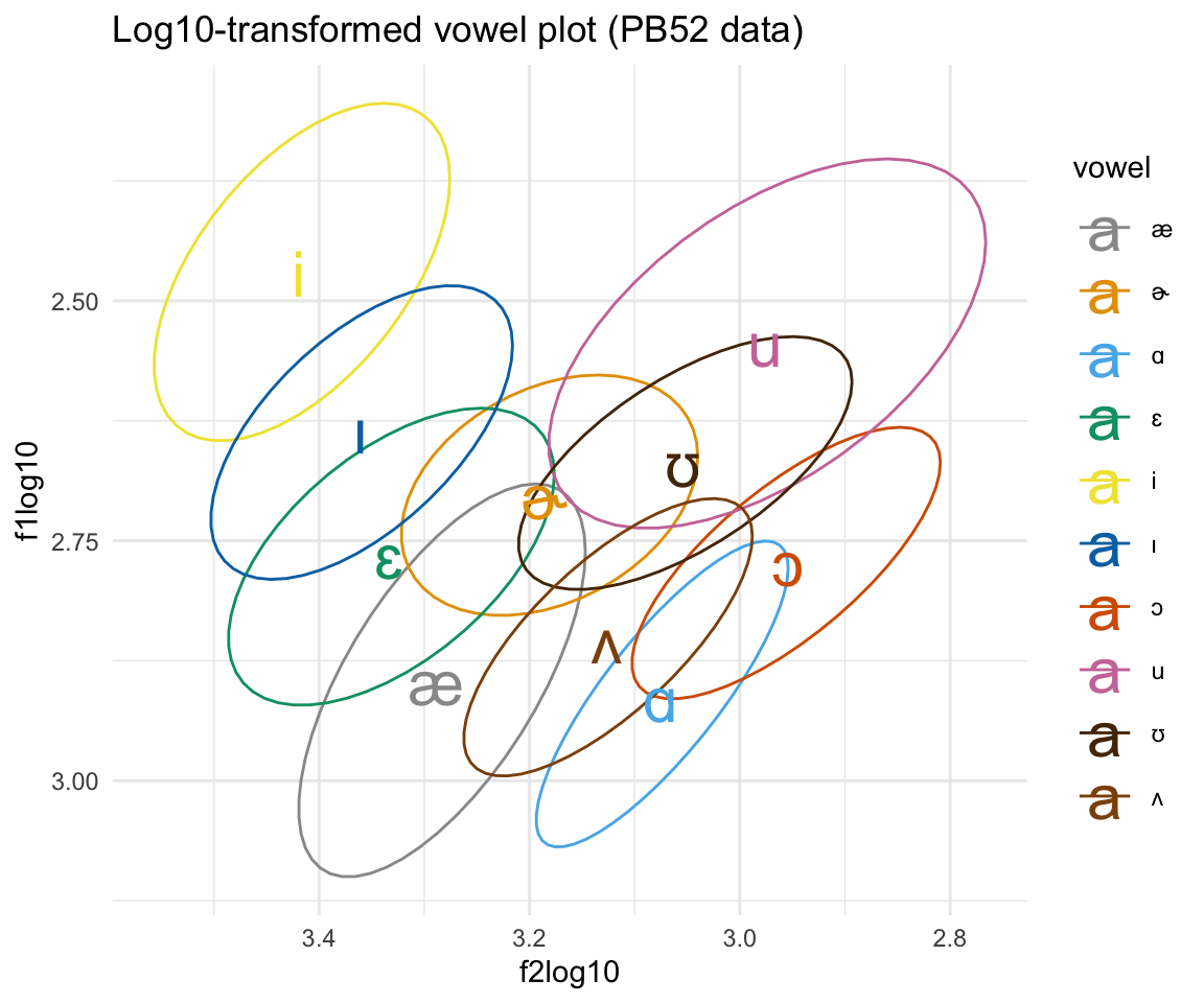
indolog = indo  %>% mutate(f1log = log(f1), f2log = log(f2), f1log10 = log10(f1), f2log10 = log10(f2))

ggplot(indolog, aes(x = f2log, y = f1log, color = vowel)) + geom_point(aes(shape = vowel),alpha = 0.3) + stat_ellipse()+ theme_minimal() +scale_color_manual(values = cbPalette[c(1:8, 1, 2)]) + scale_x_reverse() + scale_y_reverse() + scale_shape_manual(values = 1:10)+ ggtitle("Log-transformed vowel plot (Indo data)") + facet_wrap(~subj, ncol = 2)
ggplot(indolog, aes(x = f2log, y = f1log, color = vowel))  + stat_ellipse()+ theme_minimal() +scale_color_manual(values = c(cbPalette, cbPalette10)) + scale_x_reverse() + scale_y_reverse()  + geom_text(data=indolog%>%group_by(vowel, subj) %>%
               summarise_at(vars(f1log:f2log), mean, na.rm = TRUE), aes(label = vowel), size = 8)+ ggtitle("Log-transformed vowel plot (Indo data)") + facet_wrap(~subj, ncol = 2)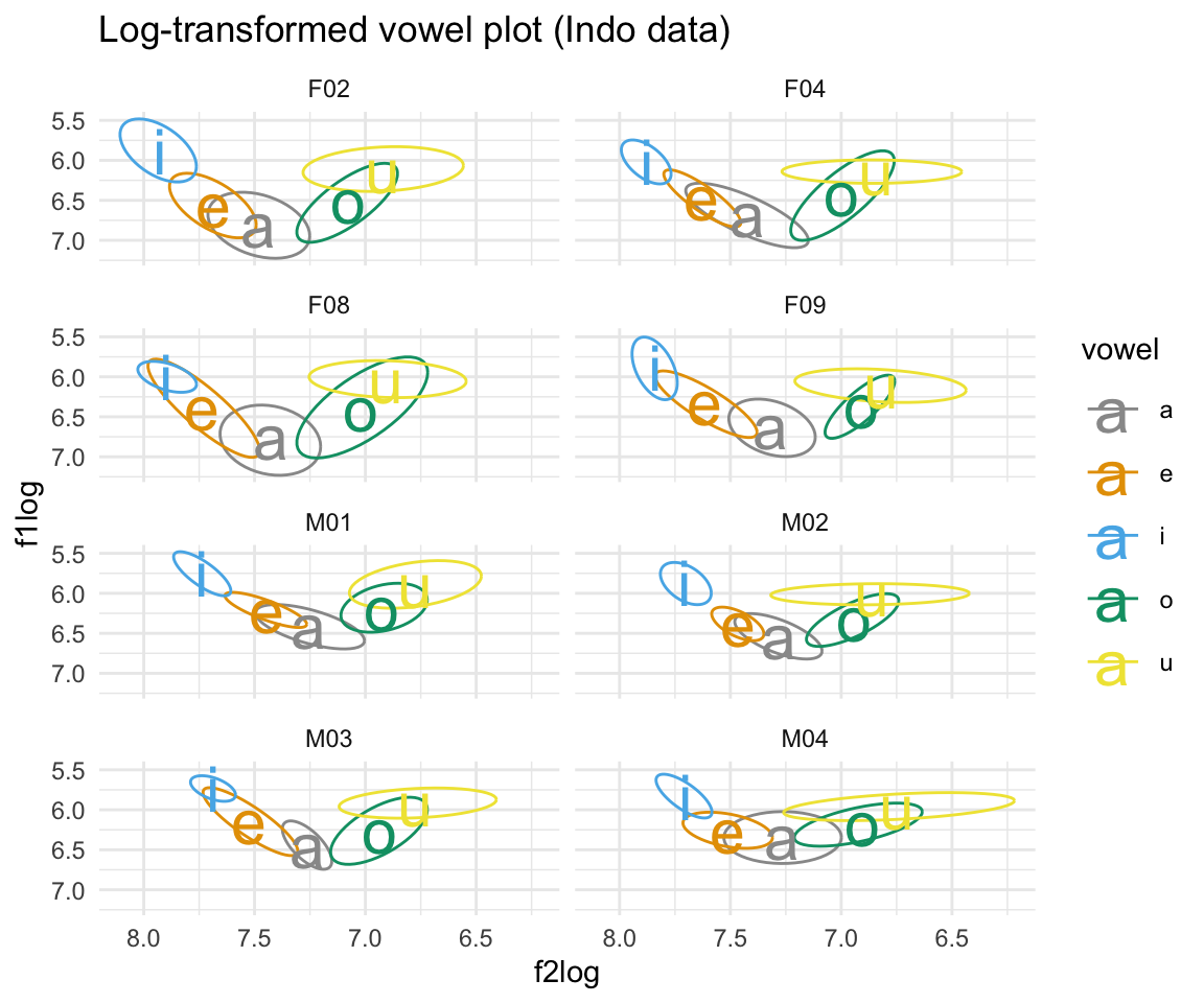
ggplot(indolog, aes(x = f2log10, y = f1log10, color = vowel)) + geom_point(aes(shape = vowel),alpha = 0.3) + stat_ellipse()+ theme_minimal() +scale_color_manual(values = cbPalette[c(1:8, 1, 2)]) + scale_x_reverse() + scale_y_reverse() + scale_shape_manual(values = 1:10) + ggtitle("Log10-transformed vowel plot (Indo data)") + facet_wrap(~subj, ncol = 2)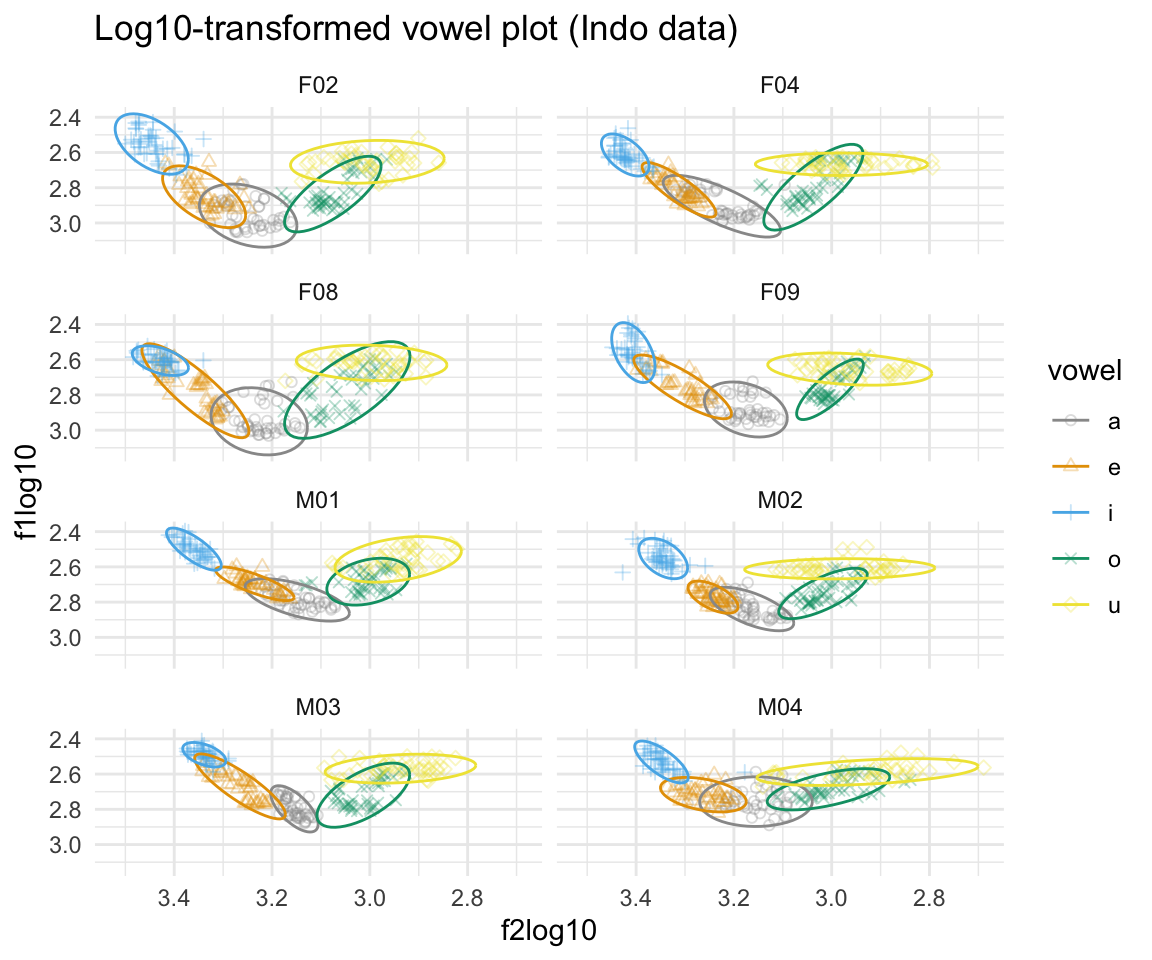
ggplot(indolog, aes(x = f2log10,y = f1log10, color = vowel))  + stat_ellipse()+ theme_minimal() +scale_color_manual(values = c(cbPalette, cbPalette10)) + scale_x_reverse() + scale_y_reverse()  + geom_text(data=indolog%>%group_by(vowel, subj) %>%
               summarise_at(vars(f1log10:f2log10), mean, na.rm = TRUE), aes(label = vowel), size = 8)+ ggtitle("Log10-transformed vowel plo (Indo data)t")+facet_wrap(~subj, ncol = 2)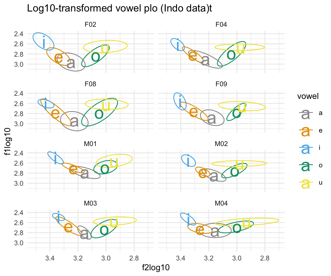
ERB
ERB (or, equivalent rectangular bandwidth), tries to approximate the bandwidths of the filtering system used in human hearing.
\[ERB = 21.4 \times log\_{10}(1+F \times 0.00437))\]
The phonR function normErb converts a given formant into ERB scale.
pb52erb = pb52 %>% mutate(f1erb = normErb(f1), f2erb = normErb(f2))
head(pb52erb)
## type sex speaker vowel repetition f0 f1 f2 f3 vowelxsampa f1erb
## 1 m m 1 i 1 160 240 2280 2850 i 6.666091
## 2 m m 1 i 2 186 280 2400 2790 i 7.427013
## 3 m m 1 ɪ 1 203 390 2030 2640 I 9.245974
## 4 m m 1 ɪ 2 192 310 1980 2550 I 7.959421
## 5 m m 1 ɛ 1 161 490 1870 2420 E 10.638141
## 6 m m 1 ɛ 2 155 570 1700 2600 E 11.618861
## f2erb
## 1 22.25500
## 2 22.68923
## 3 21.27942
## 4 21.07139
## 5 20.59663
## 6 19.81161ggplot(pb52erb, aes(x = f2erb, y = f1erb, color = vowel)) + geom_point(aes(shape = vowel),alpha = 0.3) + stat_ellipse()+ theme_minimal() +scale_color_manual(values = cbPalette[c(1:8, 1, 2)]) + scale_x_reverse() + scale_y_reverse() + scale_shape_manual(values = 1:10)+ ggtitle("ERB-transformed vowel plot (PB52 data)")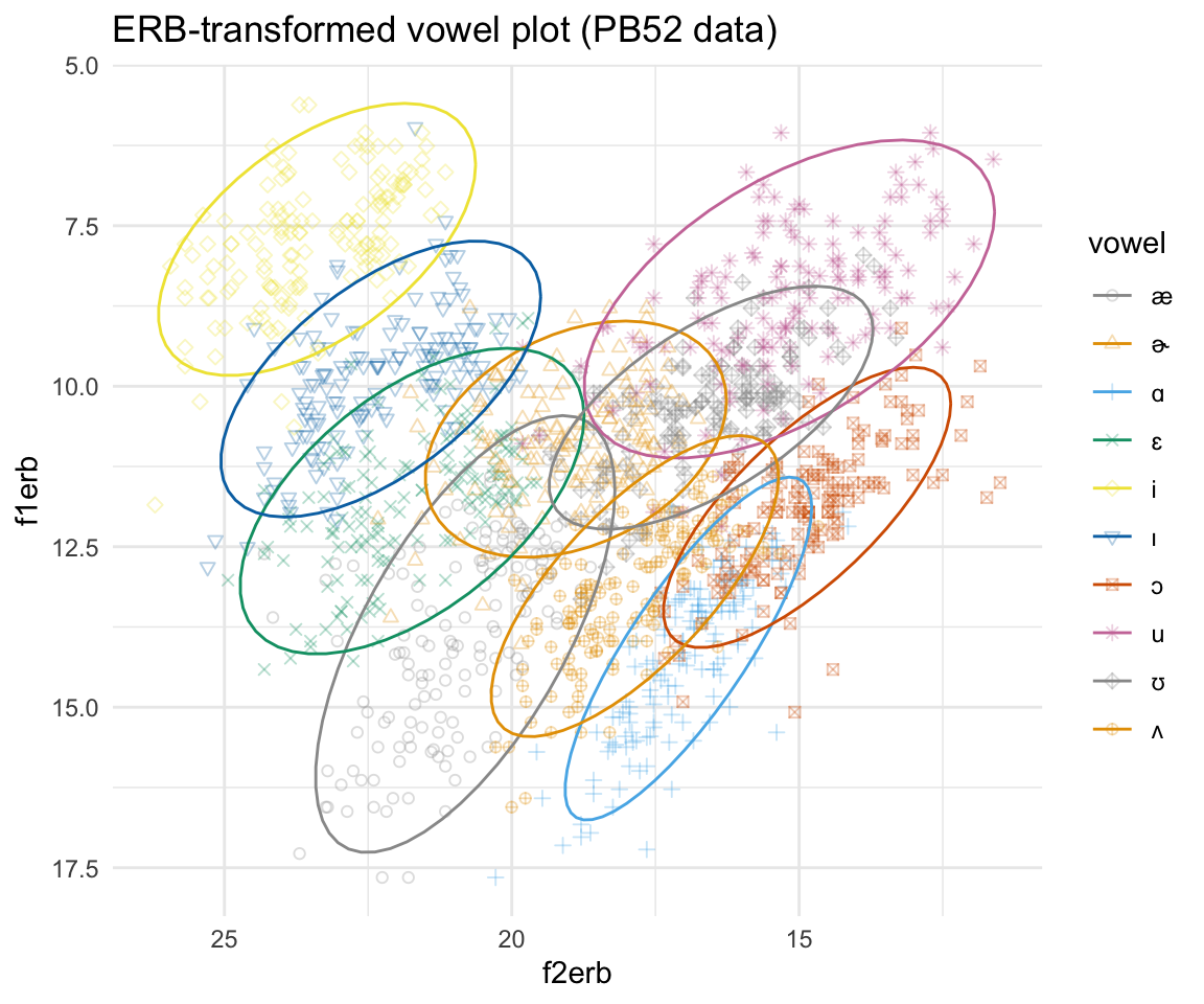
ggplot(pb52erb, aes(x = f2erb, y = f1erb, color = vowel))  + stat_ellipse()+ theme_minimal() +scale_color_manual(values = c(cbPalette, cbPalette10)) + scale_x_reverse() + scale_y_reverse()  + geom_text(data=pb52erb%>%group_by(vowel) %>%
               summarise_at(vars(f1erb:f2erb), mean, na.rm = TRUE), aes(label = vowel), size = 8)+ ggtitle("ERB-transformed vowel plot (PB52 data)")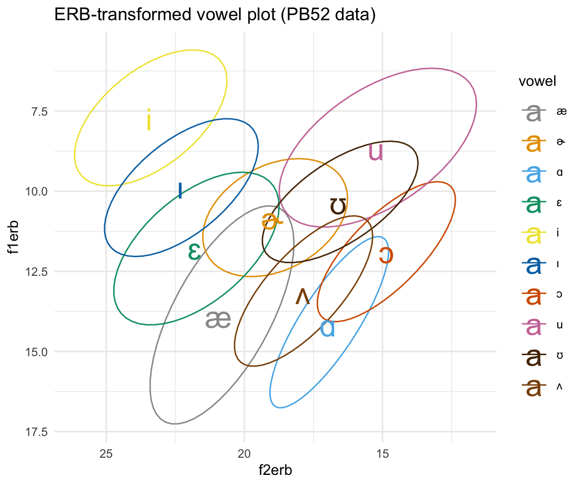
Bark
The Bark scale also tries to approximate the bandwidths of the filtering system used in human hearing.
\[Bark = \frac{26.81 \times F}{1960 + F} - 0.53\]
pb52bark = pb52 %>% mutate(f1bark = normBark(f1), f2bark = normBark(f2))
head(pb52bark)
## type sex speaker vowel repetition f0 f1 f2 f3 vowelxsampa f1bark
## 1 m m 1 i 1 160 240 2280 2850 i 2.394727
## 2 m m 1 i 2 186 280 2400 2790 i 2.821250
## 3 m m 1 ɪ 1 203 390 2030 2640 I 3.919319
## 4 m m 1 ɪ 2 192 310 1980 2550 I 3.131278
## 5 m m 1 ɛ 1 161 490 1870 2420 E 4.832000
## 6 m m 1 ɛ 2 155 570 1700 2600 E 5.510198
## f2bark
## 1 13.88670
## 2 14.22780
## 3 13.11018
## 4 12.94305
## 5 12.56000
## 6 11.92273ggplot(pb52bark, aes(x = f2bark, y = f1bark, color = vowel)) + geom_point(aes(shape = vowel),alpha = 0.3) + stat_ellipse()+ theme_minimal() +scale_color_manual(values = cbPalette[c(1:8, 1, 2)]) + scale_x_reverse() + scale_y_reverse() + scale_shape_manual(values = 1:10)+ ggtitle("bark-transformed vowel plot (PB52 data)")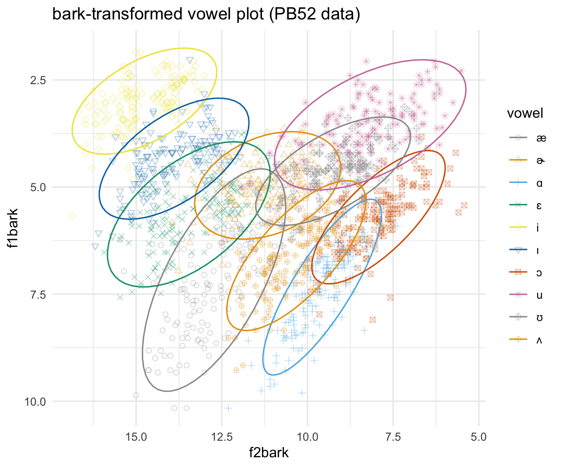
ggplot(pb52bark, aes(x = f2bark, y = f1bark, color = vowel))  + stat_ellipse()+ theme_minimal() +scale_color_manual(values = c(cbPalette, cbPalette10)) + scale_x_reverse() + scale_y_reverse()  + geom_text(data=pb52bark%>%group_by(vowel) %>%
               summarise_at(vars(f1bark:f2bark), mean, na.rm = TRUE), aes(label = vowel), size = 8)+ ggtitle("bark-transformed vowel plot (PB52 data)")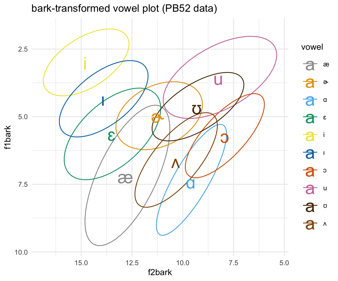
indobark = indo %>% mutate(f1bark = normBark(f1), f2bark = normBark(f2))
head(indobark)
## subj gender vowel f1 f2 f1bark f2bark
## 1 F02 f a 1052 1800 8.833918 12.30457
## 2 F02 f a 904 1911 7.932374 12.70532
## 3 F02 f a 606 1829 5.801590 12.41154
## 4 F02 f a 652 1901 6.162236 12.67016
## 5 F02 f a 1129 1863 9.268799 12.53488
## 6 F02 f a 968 1699 8.333415 11.91881ggplot(indobark, aes(x = f2bark, y = f1bark, color = vowel)) + geom_point(aes(shape = vowel),alpha = 0.3) + stat_ellipse()+ theme_minimal() +scale_color_manual(values = cbPalette[c(1:8, 1, 2)]) + scale_x_reverse() + scale_y_reverse() + scale_shape_manual(values = 1:10)+ ggtitle("bark-transformed vowel plot (Indo data)")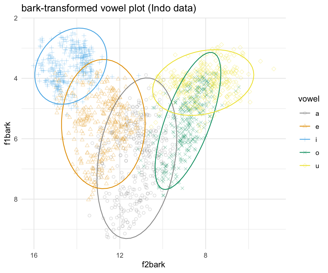
ggplot(indobark, aes(x = f2bark, y = f1bark, color = vowel))  + stat_ellipse()+ theme_minimal() +scale_color_manual(values = c(cbPalette, cbPalette10)) + scale_x_reverse() + scale_y_reverse()  + geom_text(data=indobark%>%group_by(vowel, subj) %>%
               summarise_at(vars(f1bark:f2bark), mean, na.rm = TRUE), aes(label = vowel), size = 8)+ ggtitle("bark-transformed vowel plot (Indo data)") + facet_wrap(~subj, ncol = 2)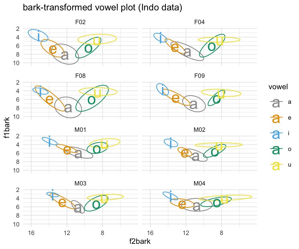
Mel
The Mel scale was originally developed as a perceptual scale of pitches judged by listeners to be equal in distance from one another. It was originally developed as a musical perceptual scale, but was extended to f0 and other formants.
\[Mel = 2595 \times log\_{10}(1 + \frac{F}{700})\]
pb52mel = pb52 %>% mutate(f1mel = normMel(f1), f2mel = normMel(f2))
head(pb52mel)
## type sex speaker vowel repetition f0 f1 f2 f3 vowelxsampa f1mel
## 1 m m 1 i 1 160 240 2280 2850 i 332.2374
## 2 m m 1 i 2 186 280 2400 2790 i 379.2023
## 3 m m 1 ɪ 1 203 390 2030 2640 I 499.0923
## 4 m m 1 ɪ 2 192 310 1980 2550 I 413.1846
## 5 m m 1 ɛ 1 161 490 1870 2420 E 598.0150
## 6 m m 1 ɛ 2 155 570 1700 2600 E 671.3412
## f2mel
## 1 1632.562
## 2 1677.054
## 3 1533.813
## 4 1512.980
## 5 1465.747
## 6 1388.619ggplot(pb52mel, aes(x = f2mel, y = f1mel, color = vowel)) + geom_point(aes(shape = vowel),alpha = 0.3) + stat_ellipse()+ theme_minimal() +scale_color_manual(values = cbPalette[c(1:8, 1, 2)]) + scale_x_reverse() + scale_y_reverse() + scale_shape_manual(values = 1:10)+ ggtitle("mel-transformed vowel plot (PB52 data)")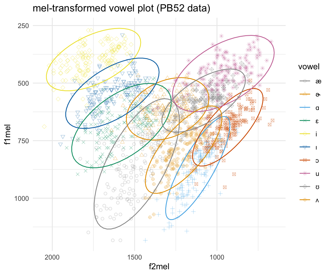
ggplot(pb52mel, aes(x = f2mel, y = f1mel, color = vowel))  + stat_ellipse()+ theme_minimal() +scale_color_manual(values = c(cbPalette, cbPalette10)) + scale_x_reverse() + scale_y_reverse()  + geom_text(data=pb52mel%>%group_by(vowel) %>%
               summarise_at(vars(f1mel:f2mel), mean, na.rm = TRUE), aes(label = vowel), size = 8)+ ggtitle("mel-transformed vowel plot (PB52 data)")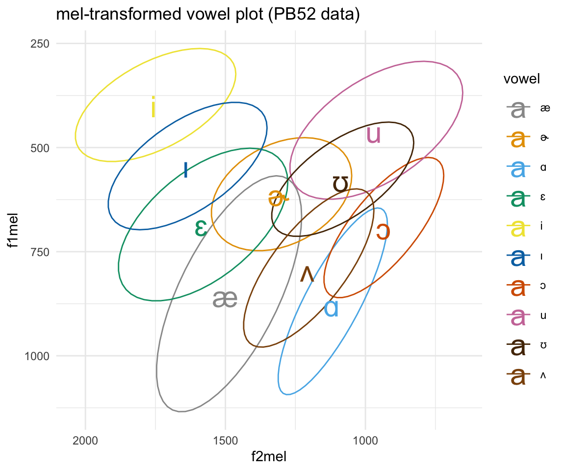
indomel = indo %>% mutate(f1mel = normMel(f1), f2mel = normMel(f2))
head(indomel)
## subj gender vowel f1 f2 f1mel f2mel
## 1 F02 f a 1052 1800 1033.9416 1434.625
## 2 F02 f a 904 1911 934.4759 1483.584
## 3 F02 f a 606 1829 702.8431 1447.623
## 4 F02 f a 652 1901 741.8551 1479.260
## 5 F02 f a 1129 1863 1082.4152 1462.673
## 6 F02 f a 968 1699 978.5693 1388.149ggplot(indomel, aes(x = f2mel, y = f1mel, color = vowel)) + geom_point(aes(shape = vowel),alpha = 0.3) + stat_ellipse()+ theme_minimal() +scale_color_manual(values = cbPalette[c(1:8, 1, 2)]) + scale_x_reverse() + scale_y_reverse() + scale_shape_manual(values = 1:10)+ ggtitle("mel-transformed vowel plot (Indo data)")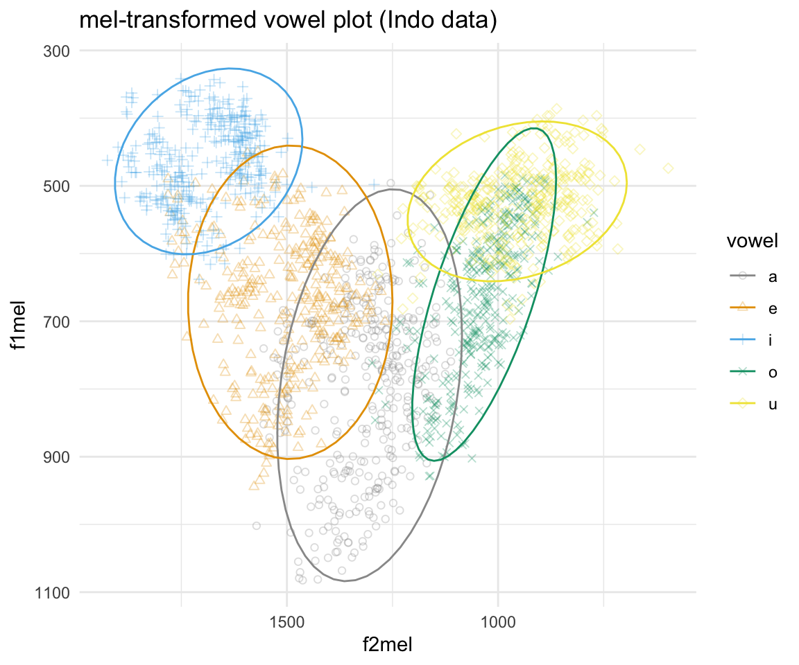
ggplot(indomel, aes(x = f2mel, y = f1mel, color = vowel))  + stat_ellipse()+ theme_minimal() +scale_color_manual(values = c(cbPalette, cbPalette10)) + scale_x_reverse() + scale_y_reverse()  + geom_text(data=indomel%>%group_by(vowel, subj) %>%
               summarise_at(vars(f1mel:f2mel), mean, na.rm = TRUE), aes(label = vowel), size = 8)+ ggtitle("mel-transformed vowel plot (Indo data)") + facet_wrap(~subj, ncol = 2)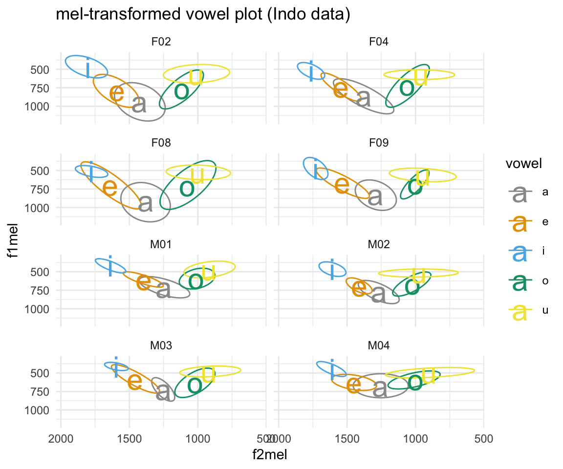
Speaker intrinsic/vowel intrinsic/formant extrinsic
Speaker intrinsic and formant extrinsic methods use multiple formants in order to calculate normalized values. The most common one is the Bark-distance model.
Bark distance model
The Bark distance model was proposed by Syrdal and Gopal (1986). In this model, F0-F3 are transformed into bark scale. Following this, \[F1\prime\] is calculated as the difference: \[F1\_{bark} - F0\_{bark}\], and \[F2\prime\] is calculated as the difference: \[F3\_{bark} - F2\_{bark}\]. Unfortunately, there is no function to do this calculation directly, so we will use the normBark function and calculate the differences ourselves. Note that the Peterson and Barney data has f0-F3 information, whereas the indo data only has F1-F2.
pb52SG = pb52 %>% mutate(f0bark = normBark(f0), f1bark = normBark(f1), f2bark = normBark(f2), f3bark = normBark(f3), f1new = f1bark-f0bark, f2new = f3bark-f2bark)

ggplot(pb52SG, aes(x = f2new, y = f1new, color = vowel)) + geom_point(aes(shape = vowel),alpha = 0.3) + stat_ellipse()+ theme_minimal() +scale_color_manual(values = cbPalette[c(1:8, 1, 2)]) + scale_x_reverse() + scale_y_reverse() + scale_shape_manual(values = 1:10)+ ggtitle("SG-transformed vowel plot (PB52 data)")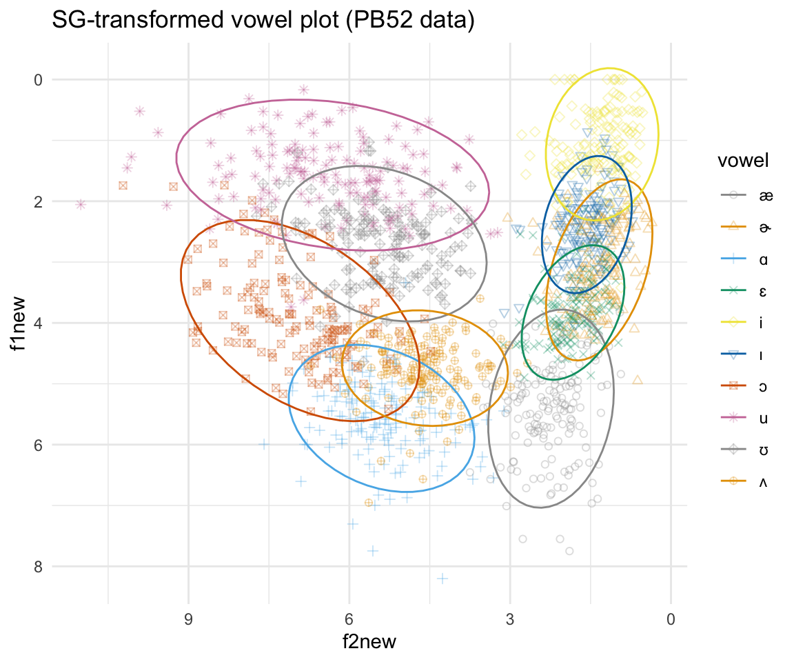
ggplot(pb52SG, aes(x = f2new, y = f1new, color = vowel))  + stat_ellipse()+ theme_minimal() +scale_color_manual(values = c(cbPalette, cbPalette10)) + scale_y_reverse()  + geom_text(data=pb52SG%>%group_by(vowel) %>%
               summarise_at(vars(f1new:f2new), mean, na.rm = TRUE), aes(label = vowel), size = 8)+ ggtitle("SG-transformed vowel plot (PB52 data)")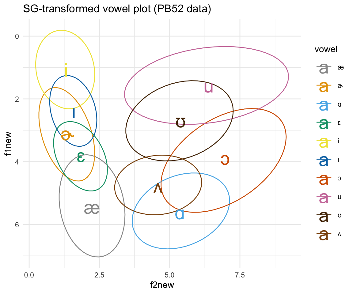
set.seed(13579)

pb52SGsample = pb52SG %>% filter(speaker %in% sample(levels(pb52SG$speaker), 10, replace = FALSE))

ggplot(pb52SGsample, aes(x = f2new, y = f1new, color = vowel)) +theme_minimal() +scale_color_manual(values = c(cbPalette, cbPalette10)) + scale_y_reverse()  +facet_wrap(~speaker) + geom_text(data=pb52SGsample%>%group_by(vowel, speaker) %>% summarise_at(vars(f1new:f2new), mean, na.rm = TRUE), aes(label = vowel), size = 8)+ ggtitle("SG-transformed vowel plot (10 speakers from the PB52 data)")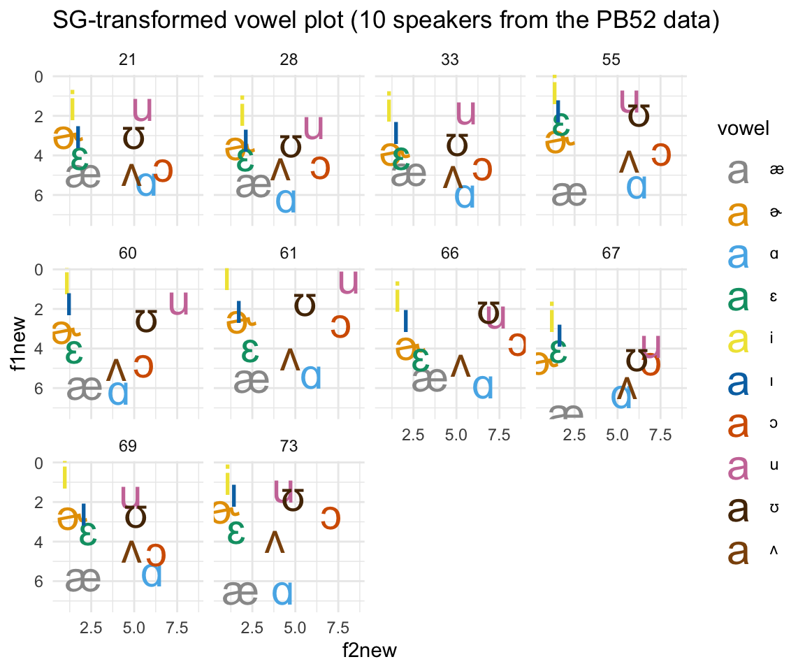
Speaker intrinsic/vowel extrinsic/formant intrinsic
Vowel extrinsic, formant intrinsic models are often used for sociophonetic purposes. These take into account all vowels in a system simultaneously, but only use one formant at a time.
Z-score/Lobanov normalization
The use of z-score as a method of vowel normalization was first introduced by Lobanov (1971). In this method, each subject’s formants are put on a scale of standard deviations.
\[F\_i = \frac{F\_i-\mu(F\_i)}{\sigma(F\_i)}\]
This can be done using either the normLobanov() function from phonR or the scale() function in base R.
pb52lobanov = pb52 %>% group_by(speaker) %>% mutate(f1scale = scale(f1), f2scale = scale(f2), f1lobanov = normLobanov(f1), f2lobanov = normLobanov(f2))

#to show that these two functions do the same thing
all.equal(pb52lobanov$f1lobanov, pb52lobanov$f1scale)
## [1] TRUEall.equal(pb52lobanov$f2lobanov, pb52lobanov$f2scale)## [1] TRUEggplot(pb52lobanov, aes(x = f2lobanov, y = f1lobanov, color = vowel)) + geom_point(aes(shape = vowel),alpha = 0.3) + stat_ellipse()+ theme_minimal() +scale_color_manual(values = cbPalette[c(1:8, 1, 2)]) + scale_x_reverse() + scale_y_reverse() + scale_shape_manual(values = 1:10)+ ggtitle("Lobanov-transformed vowel plot (PB52 data)")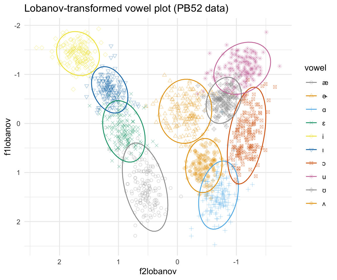
ggplot(pb52lobanov, aes(x = f2lobanov, y = f1lobanov, color = vowel))  + stat_ellipse()+ theme_minimal() +scale_color_manual(values = c(cbPalette, cbPalette10)) + scale_y_reverse() + scale_x_reverse()  + geom_text(data=pb52lobanov%>%group_by(vowel) %>%
               summarise_at(vars(f1lobanov:f2lobanov), mean, na.rm = TRUE), aes(label = vowel), size = 8)+ ggtitle("Lobanov-transformed vowel plot (PB52 data)")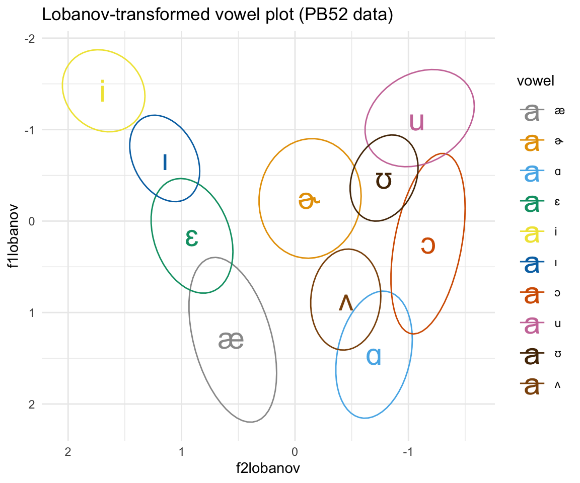
set.seed(13579)

pb52lobanovsample = pb52lobanov %>% filter(speaker %in% sample(levels(pb52lobanov$speaker), 10, replace = FALSE))

ggplot(pb52lobanovsample, aes(x = f2lobanov, y = f1lobanov, color = vowel))  +theme_minimal() +scale_color_manual(values = c(cbPalette, cbPalette10)) + scale_y_reverse() +scale_x_reverse() +facet_wrap(~speaker) + geom_text(data=pb52lobanovsample%>%group_by(vowel, speaker) %>% summarise_at(vars(f1lobanov:f2lobanov), mean, na.rm = TRUE), aes(label = vowel), size = 8)+ ggtitle("lobanov-transformed vowel plot (10 speakers from the PB52 data)")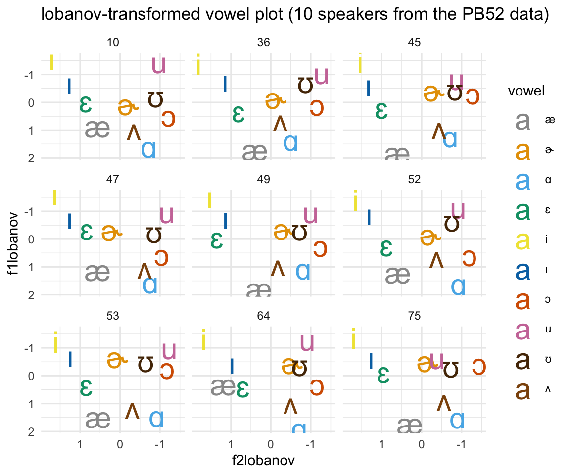
Individual log means (Nearey1)
Note that Terrance Nearey, in his 1978 dissertation, created two methods for vowel normalization. Both are vowel extrinsic. This method is formant intrinsic. I will discuss the formant extrinsic method below. The method described here is useful for sociophonetic purposes, and has been considered by many to be the most successful in maintaining sociophonetic data during normalization.
\[F\_n\prime = log\_e(F\_n) - \mu(log\_e(F\_n))\]
Note that F1 and F2 are required for this method as an input.
pb52nearey1 = with(pb52, normNearey1(cbind(f1, f2), group = speaker))
colnames(pb52nearey1) = c("f1nearey1", "f2nearey1")
pb52nearey1 = cbind(pb52, pb52nearey1)

ggplot(pb52nearey1, aes(x = f2nearey1, y = f1nearey1, color = vowel)) + geom_point(aes(shape = vowel),alpha = 0.3) + stat_ellipse()+ theme_minimal() +scale_color_manual(values = cbPalette[c(1:8, 1, 2)]) + scale_x_reverse() + scale_y_reverse() + scale_shape_manual(values = 1:10)+ ggtitle("nearey1-transformed vowel plot (PB52 data)")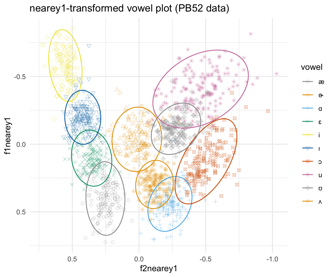
ggplot(pb52nearey1, aes(x = f2nearey1, y = f1nearey1, color = vowel))  + stat_ellipse()+ theme_minimal() +scale_color_manual(values = c(cbPalette, cbPalette10)) + scale_y_reverse() + scale_x_reverse()  + geom_text(data=pb52nearey1%>%group_by(vowel) %>%
               summarise_at(vars(f1nearey1:f2nearey1), mean, na.rm = TRUE), aes(label = vowel), size = 8)+ ggtitle("nearey1-transformed vowel plot (PB52 data)")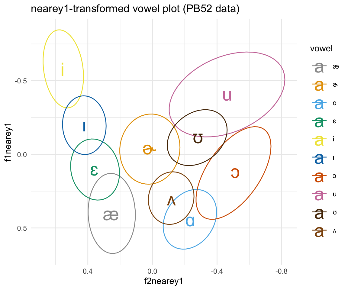
set.seed(13579)

pb52nearey1sample = pb52nearey1 %>% filter(speaker %in% sample(levels(pb52nearey1$speaker), 10, replace = FALSE))

ggplot(pb52nearey1sample, aes(x = f2nearey1, y = f1nearey1, color = vowel))  +theme_minimal() +scale_color_manual(values = c(cbPalette, cbPalette10)) + scale_y_reverse() +scale_x_reverse() +facet_wrap(~speaker) + geom_text(data=pb52nearey1sample%>%group_by(vowel, speaker) %>% summarise_at(vars(f1nearey1:f2nearey1), mean, na.rm = TRUE), aes(label = vowel), size = 8)+ ggtitle("nearey1-transformed vowel plot (10 speakers from the PB52 data)")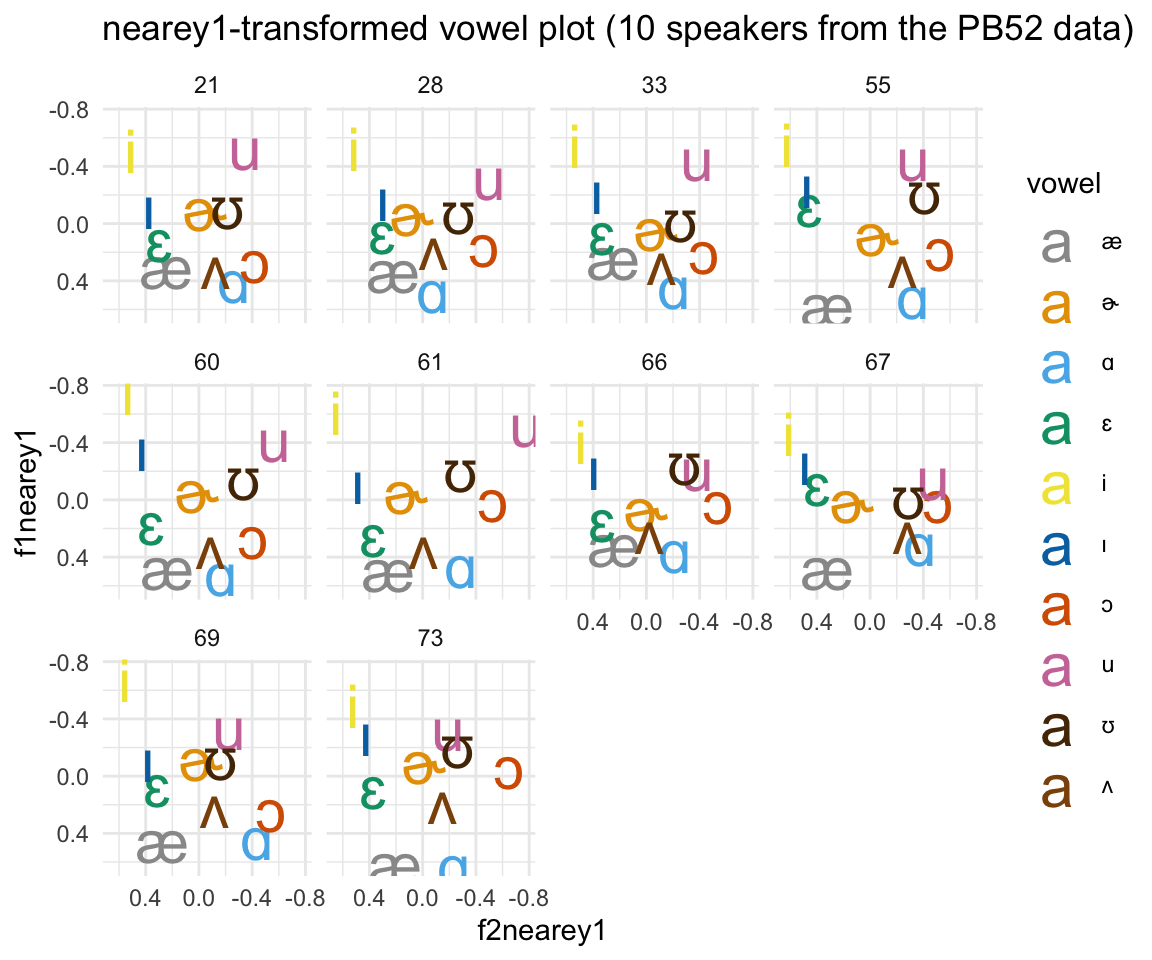
Centroids (Watt-Fabricius)
The Watt and Fabricius method is vowel extrinsic, but unlike other methods, the centroid used to calculate normalized values is based on points that represent the corners of the vowel space (/a/, /i/, and /u/).
\[<F1\prime, F2\prime> = <\frac{2\times F2}{min(\mu\times F2\_v) +max(\mu\times F2\_v)}, \frac{3\times F1}{2 \times min(\mu\times F1\_v) +max(\mu\times F1\_v)}>\]
Note that the implementation of this method used in phonR calculates “which vowel has the highest mean F2 value and uses that to calculate the upper left corner, rather than expressly looking for the mean of the”point vowel” /i/. The upper right corner is, as in the original method, derived from the other two. If the vowels with the highest mean F1 and highest mean F2 are not the same pair of vowels for all members of group, normWattFabricius returns an error.” (quote taken from the phonR help page)
pb52WF = with(pb52, normWattFabricius(cbind(f1, f2), group = speaker, vowel = vowel))## [phonR]: The vowel with the lowest mean F1 value (usually /i/)does not match across all speakers/groups. You'll have to calculate s-centroid manually.## Warning in data.frame(minF1 = minima["f1", ], vowel = dimnames(means)[[1]]
## [min.id["f1", : row names were found from a short variable and have been
## discarded## minF1.f1 minF1.f2 vowel group
## 1 NA NA u 1
## 2 NA NA i 2
## 3 NA NA i 3
## 4 NA NA i 4
## 5 NA NA i 5
## 6 NA NA u 6
## 7 NA NA i 7
## 8 NA NA i 8
## 9 NA NA i 9
## 10 NA NA i 10
## 11 NA NA i 11
## 12 NA NA i 12
## 13 NA NA i 13
## 14 NA NA i 14
## 15 NA NA i 15
## 16 NA NA i 16
## 17 NA NA i 17
## 18 NA NA i 18
## 19 NA NA i 19
## 20 NA NA i 20
## 21 NA NA u 21
## 22 NA NA u 22
## 23 NA NA i 23
## 24 NA NA i 24
## 25 NA NA i 25
## 26 NA NA i 26
## 27 NA NA i 27
## 28 NA NA i 28
## 29 NA NA u 29
## 30 NA NA i 30
## 31 NA NA i 31
## 32 NA NA i 32
## 33 NA NA i 33
## 34 NA NA i 34
## 35 NA NA i 35
## 36 NA NA i 36
## 37 NA NA i 37
## 38 NA NA i 38
## 39 NA NA i 39
## 40 NA NA i 40
## 41 NA NA i 41
## 42 NA NA i 42
## 43 NA NA i 43
## 44 NA NA i 44
## 45 NA NA i 45
## 46 NA NA i 46
## 47 NA NA i 47
## 48 NA NA u 48
## 49 NA NA i 49
## 50 NA NA u 50
## 51 NA NA u 51
## 52 NA NA i 52
## 53 NA NA i 53
## 54 NA NA i 54
## 55 NA NA i 55
## 56 NA NA i 56
## 57 NA NA i 57
## 58 NA NA i 58
## 59 NA NA i 59
## 60 NA NA i 60
## 61 NA NA i 61
## 62 NA NA u 62
## 63 NA NA i 63
## 64 NA NA i 64
## 65 NA NA i 65
## 66 NA NA i 66
## 67 NA NA i 67
## 68 NA NA i 68
## 69 NA NA i 69
## 70 NA NA i 70
## 71 NA NA i 71
## 72 NA NA i 72
## 73 NA NA i 73
## 74 NA NA i 74
## 75 NA NA i 75
## 76 NA NA i 76## Error in normWattFabricius(cbind(f1, f2), group = speaker, vowel = vowel):Therefore, for simplicity, we will use the phonTools function normalize().
pb52WF = with(pb52, normalize(cbind(f1, f2), speaker, vowel,method = 'wandf', corners = c('i','u')))
head(pb52WF)
## f1 f2 speaker vowel
## 1 0.9290323 1.907950 1 i
## 2 1.0838710 2.008368 1 i
## 3 1.5096774 1.698745 1 ɪ
## 4 1.2000000 1.656904 1 ɪ
## 5 1.8967742 1.564854 1 ɛ
## 6 2.2064516 1.422594 1 ɛggplot(pb52WF, aes(x = f2, y = f1, color = vowel)) + geom_point(aes(shape = vowel),alpha = 0.3) + stat_ellipse()+ theme_minimal() +scale_color_manual(values = cbPalette[c(1:8, 1, 2)]) + scale_x_reverse() + scale_y_reverse() + scale_shape_manual(values = 1:10)+ ggtitle("Watt-Fabricius-transformed vowel plot (PB52 data)")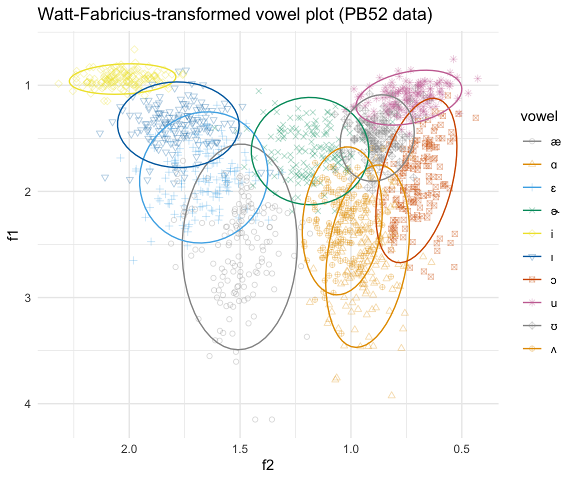
ggplot(pb52WF, aes(x = f2, y = f1, color = vowel))  + stat_ellipse()+ theme_minimal() +scale_color_manual(values = c(cbPalette, cbPalette10)) + scale_y_reverse() + scale_x_reverse()  + geom_text(data=pb52WF%>%group_by(vowel)%>%
               summarise_at(vars(f1:f2), mean, na.rm = TRUE), aes(label = vowel), size = 8)+ ggtitle("Watt-Fabricius-transformed vowel plot (PB52 data)")
set.seed(13579)

pb52WFsample = pb52WF %>% filter(speaker %in% sample(levels(pb52WF$speaker), 10, replace = FALSE))

ggplot(pb52WFsample, aes(x = f2, y = f1, color = vowel))  +theme_minimal() +scale_color_manual(values = c(cbPalette, cbPalette10)) + scale_y_reverse() +scale_x_reverse() +facet_wrap(~speaker) + geom_text(data=pb52WFsample%>%group_by(vowel, speaker) %>% summarise_at(vars(f1:f2), mean, na.rm = TRUE), aes(label = vowel), size = 8)+ ggtitle("WF-transformed vowel plot (10 speakers from the PB52 data)")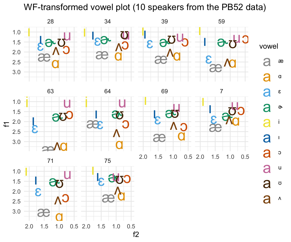
Speaker intrinsic/vowel extrinsic/formant extrinsic
Shared log-mean (Nearey2)
This method is similar to the Nearey1 method above, except rather than calculating the logmean for an individual vowel formant, it calculates the logmean for all formants.
\[F\_n = F\_n - (\mu\_0 + \mu\_1 + \mu\_2 + \mu\_3)\] where \[\mu\_n\] is the log mean for f0-F3.
pb52nearey2 = with(pb52, normNearey2(cbind(f0, f1, f2, f3), group = speaker))
head(pb52nearey2)
## f0 f1 f2 f3
## 1 -1.485579 -1.0801136 1.1711782 1.394322
## 2 -1.335006 -0.9259629 1.2224715 1.373044
## 3 -1.247547 -0.5946058 1.0550385 1.317782
## 4 -1.303257 -0.8241802 1.0300996 1.283096
## 5 -1.479348 -0.3663471 0.9729412 1.230770
## 6 -1.517327 -0.2151162 0.8776310 1.302514colnames(pb52nearey2) = c("f0nearey2", "f1nearey2", "f2nearey2", "f3nearey2")
pb52nearey2 = cbind(pb52, pb52nearey2)
ggplot(pb52nearey2, aes(x = f2nearey2, y = f1nearey2, color = vowel)) + geom_point(aes(shape = vowel),alpha = 0.3) + stat_ellipse()+ theme_minimal() +scale_color_manual(values = cbPalette[c(1:8, 1, 2)]) + scale_x_reverse() + scale_y_reverse() + scale_shape_manual(values = 1:10)+ ggtitle("nearey2-transformed vowel plot (PB52 data)")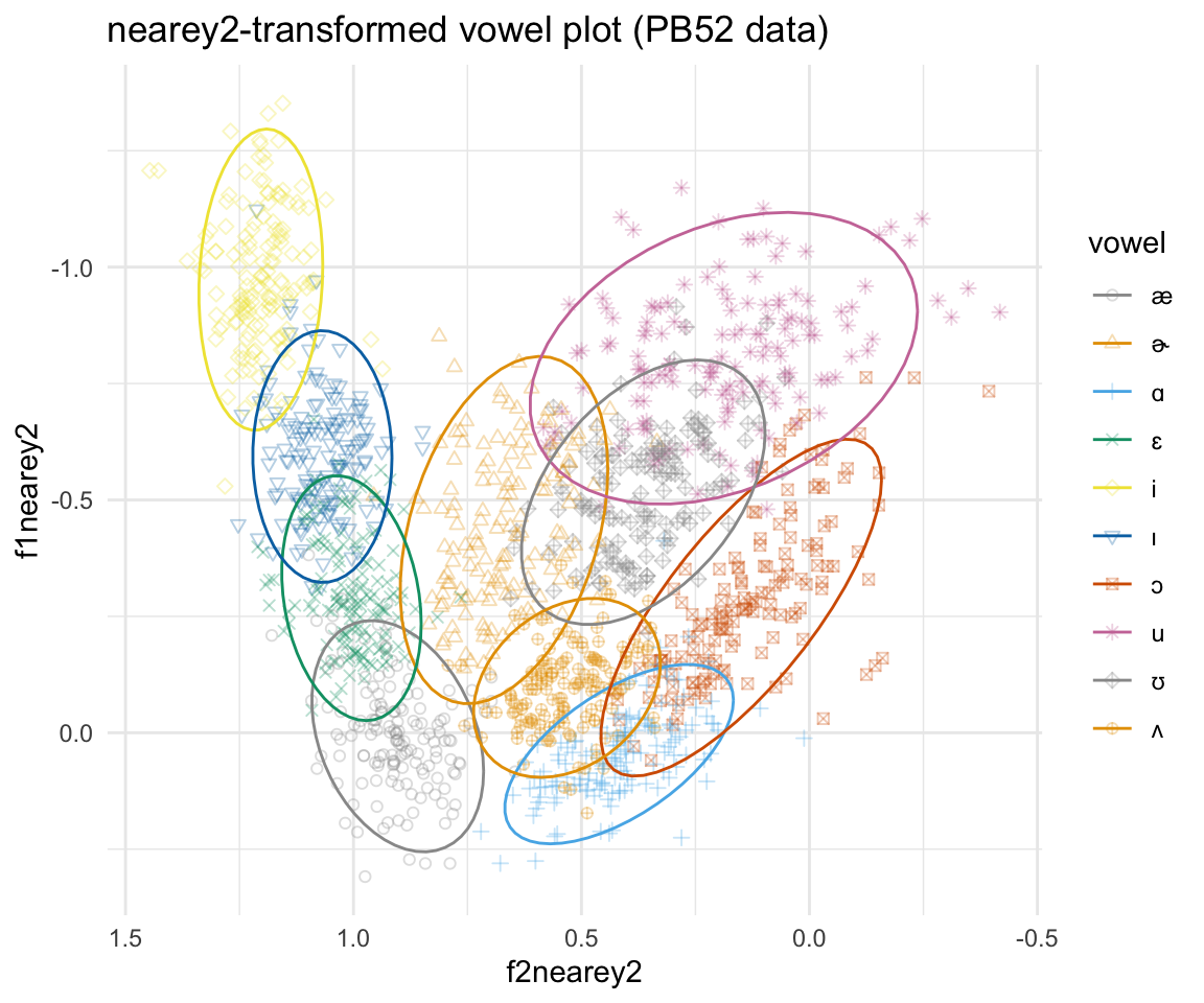
ggplot(pb52nearey2, aes(x = f2nearey2, y = f1nearey2, color = vowel))  + stat_ellipse()+ theme_minimal() +scale_color_manual(values = c(cbPalette, cbPalette10)) + scale_y_reverse() + scale_x_reverse()  + geom_text(data=pb52nearey2%>%group_by(vowel) %>%
               summarise_at(vars(f1nearey2:f2nearey2), mean, na.rm = TRUE), aes(label = vowel), size = 8)+ ggtitle("nearey2-transformed vowel plot (PB52 data)")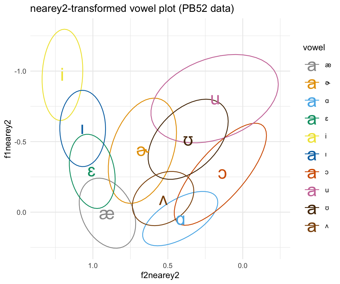
set.seed(13579)

pb52nearey2sample = pb52nearey2 %>% filter(speaker %in% sample(levels(pb52nearey2$speaker), 10, replace = FALSE))

ggplot(pb52nearey2sample, aes(x = f2nearey2, y = f1nearey2, color = vowel))  +theme_minimal() +scale_color_manual(values = c(cbPalette, cbPalette10)) + scale_y_reverse() +scale_x_reverse() +facet_wrap(~speaker) + geom_text(data=pb52nearey2sample%>%group_by(vowel, speaker) %>% summarise_at(vars(f1nearey2:f2nearey2), mean, na.rm = TRUE), aes(label = vowel), size = 8)+ ggtitle("nearey2-transformed vowel plot (10 speakers from the PB52 data)")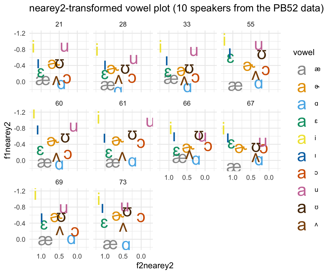
Speaker extrinsic/vowel extrinsic/formant extrinsic
ANAE method
This is the normalization method used by the phonological Atlas of North American English (Labov et al. 2006) - is a modification of Nearey2.
While it also uses a log-mean method to normalize the formant values, the primary difference is that it computes a single grand mean for all speakers included in the study (i.e. it’s speaker-extrinsic, while Nearey is typically speaker-intrinsic). Also, unlike Nearey, it computes a scaling factor for each individual which is then used to modify each individual’s vowel space rather than computing a set of non-Hertz-like values. In other words, since it is speaker-extrinsic, it is able to scale the original Hertz values as a part of its normalization process. source
Note that Labov said when writing about this method that it took up to 350 speakers before the sliding mean would change, so it is unlikely we will be using this method in our current research.
Note that the vowels package is the only one that does this method, as far as I am aware. The data needs to be in a very specific format in order to work properly:
pb52ANAE = pb52 %>% mutate(F1_glide = NA, F2_glide = NA, F3_glide = NA, context = NA)
head(pb52ANAE)
## type sex speaker vowel repetition f0 f1 f2 f3 vowelxsampa F1_glide
## 1 m m 1 i 1 160 240 2280 2850 i NA
## 2 m m 1 i 2 186 280 2400 2790 i NA
## 3 m m 1 ɪ 1 203 390 2030 2640 I NA
## 4 m m 1 ɪ 2 192 310 1980 2550 I NA
## 5 m m 1 ɛ 1 161 490 1870 2420 E NA
## 6 m m 1 ɛ 2 155 570 1700 2600 E NA
## F2_glide F3_glide context
## 1 NA NA NA
## 2 NA NA NA
## 3 NA NA NA
## 4 NA NA NA
## 5 NA NA NA
## 6 NA NA NAcolnames(pb52ANAE)[c(3, 4, 6:9)] = c("speaker_id", "vowel_id", "F0", "F1", "F2", "F3")
pb52ANAE = pb52ANAE %>% select(speaker_id, vowel_id, context, F1, F2, F3, F1_glide, F2_glide, F3_glide)
pb52ANAE_out = norm.labov(pb52ANAE, use.f3 = TRUE)
colnames(pb52ANAE_out)[4:9] = c("F1", "F2","F3", "F1glide", "F2glide", "F3glide")
ggplot(pb52ANAE_out, aes(x = F2, y = F1, color = Vowel)) + geom_point(alpha = 0.4, size = 0.4) + stat_ellipse() + scale_colour_manual(values = cbPalette10) + scale_y_reverse() + scale_x_reverse() + theme_minimal()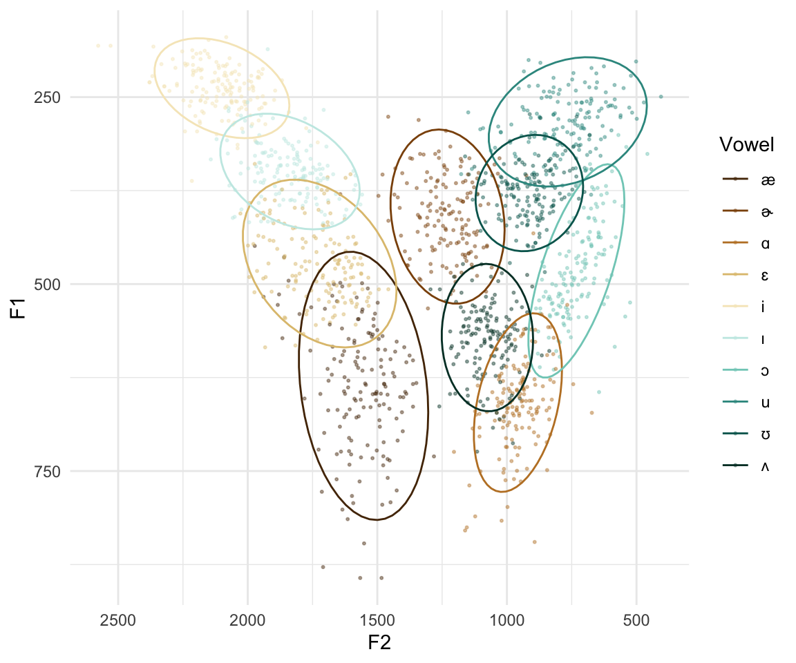
Which method is best?
Of course, after being bombarded with this information, you are probably wondering which of these is the best method to use. Adank et al. (2004) ran a series of linear discriminant analyses using these methods in order to identify the “best” method of vowel normalization. The results showed that the Lobanov method is the best procedure, though the difference with the Nearey1 method is relatively small. It is of course important to note that these methods end up with non-Hz scales of the formants, so proceed with caution!
A summary of the methods discussed above can be found here.