Text Mining with R
#Setting up an API The first thing to do with R when getting ready to do Twitter mining is to set up your credentials. I won’t go through this process right now, but it is outlined here. You need to first become a Twitter developer and create an app. It only takes a few moments.
There are a couple of different types of flows you can work with, depending on what your question is. For example, if you want to look at word counts and frequencies, your workflow will look something like this:
If you want to do sentiment analysis, your workflow will look something like this:
#Mining and Processing
##Searching for tweets
There are a number of functions/packages that allow you to search for tweets:
- searchTwitteR in the TwitteR package (I’ve had a lot of problems with this package and limitations on number of tweets allowed to be grabbed.)
- search_tweets in the rtweet package
- filterStream in the streamR package
For this example, I will show you the results from the rtweet package. Note that these packages will only give recent tweets, generally from the past week. (Note, I collected these tweets on Sept. 5, 2018.)
#This gets the 5000 most recent tweets from each of the handles listed.
timelines <- get_timelines(c("nbcsports", "cbssports", "bbcsport"), n = 5000, retryonratelimit = TRUE)

#This gets the 5000 most recent tweets that have one of the words listed. You can also use AND as a search operator to look for tweets that meet multiple criteria.
footballterms = search_tweets2(c("football OR  nfl OR superbowl", "lang:en"), n = 5000, retryonratelimit = TRUE, geocode = lookup_coords("usa"))
footballterms = lat_lng(footballterms) #gives latitude and longitude for geocodes that are given

#searching for three types of cute animals
cuteanimals = search_tweets("dog OR cat OR hamster", n = 5000, retryonratelimit = TRUE, geocode = lookup_coords("usa"))
cuteanimals = lat_lng(cuteanimals)
patterns = c("cat|dog|hamster")
#create a new variable that takes out which animal was mentioned
cuteanimals = cuteanimals %>% mutate(animalmentioned = str_extract(tolower(text), patterns))


champaign = search_tweets(n = 10000, geocode ="-88.24338, 40.11642, 5mi")
#save all files for future use

save(timelines, file = "twittertimelines.Rda")
save(footballterms, file = "footballterms.Rda")
save(cuteanimals, file = "cuteanimals.Rda")
Here’s how you would do it with the twitteR package. I personally have not had a lot of luck with this package, and I have heard it is being deprecated because of rtweets.
#CBStweets = searchTwitteR("from:@cbssports", n = 1000)
#BBCtweets = searchTwitteR("from:@bbcsport", n = 1000)
#NBCtweets = searchTwitteR("from:@nbcsports", n = 1000)
#Comparing three Twitter Users ##Processing Data
As you can see, there is a LOT of information we’re given when we download tweets. We only need a small subset of it, so we will use the tidyverse to select out the data we need, and we will forget the rest.
head(timelines)## # A tibble: 6 x 88
## user_id status_id created_at screen_name text source
## <chr> <chr> <dttm> <chr> <chr> <chr>
## 1 118563… 10371523… 2018-09-05 01:36:04 NBCSports Yasi… Spred…
## 2 118563… 10371448… 2018-09-05 01:06:05 NBCSports Kobe… Spred…
## 3 118563… 10371440… 2018-09-05 01:03:02 NBCSports Sere… Spred…
## 4 118563… 10371322… 2018-09-05 00:16:05 NBCSports Is i… Spred…
## 5 118563… 10371246… 2018-09-04 23:46:04 NBCSports Andr… Spred…
## 6 118563… 10371186… 2018-09-04 23:22:17 NBCSports PHIL… Twitt…
## # … with 82 more variables: display_text_width <dbl>, reply_to_status_id <chr>,
## # reply_to_user_id <chr>, reply_to_screen_name <chr>, is_quote <lgl>,
## # is_retweet <lgl>, favorite_count <int>, retweet_count <int>,
## # hashtags <list>, symbols <chr>, urls_url <list>, urls_t.co <list>,
## # urls_expanded_url <list>, media_url <list>, media_t.co <list>,
## # media_expanded_url <list>, media_type <list>, ext_media_url <list>,
## # ext_media_t.co <list>, ext_media_expanded_url <list>, ext_media_type <chr>,
## # mentions_user_id <list>, mentions_screen_name <list>, lang <chr>,
## # quoted_status_id <chr>, quoted_text <chr>, quoted_created_at <dttm>,
## # quoted_source <chr>, quoted_favorite_count <int>,
## # quoted_retweet_count <int>, quoted_user_id <chr>, quoted_screen_name <chr>,
## # quoted_name <chr>, quoted_followers_count <int>,
## # quoted_friends_count <int>, quoted_statuses_count <int>,
## # quoted_location <chr>, quoted_description <chr>, quoted_verified <lgl>,
## # retweet_status_id <chr>, retweet_text <chr>, retweet_created_at <dttm>,
## # retweet_source <chr>, retweet_favorite_count <int>,
## # retweet_retweet_count <int>, retweet_user_id <chr>,
## # retweet_screen_name <chr>, retweet_name <chr>,
## # retweet_followers_count <int>, retweet_friends_count <int>,
## # retweet_statuses_count <int>, retweet_location <chr>,
## # retweet_description <chr>, retweet_verified <lgl>, place_url <chr>,
## # place_name <chr>, place_full_name <chr>, place_type <chr>, country <chr>,
## # country_code <chr>, geo_coords <list>, coords_coords <list>,
## # bbox_coords <list>, status_url <chr>, name <chr>, location <chr>,
## # description <chr>, url <chr>, protected <lgl>, followers_count <int>,
## # friends_count <int>, listed_count <int>, statuses_count <int>,
## # favourites_count <int>, account_created_at <dttm>, verified <lgl>,
## # profile_url <chr>, profile_expanded_url <chr>, account_lang <chr>,
## # profile_banner_url <chr>, profile_background_url <chr>,
## # profile_image_url <chr>dim(timelines)## [1] 8827 88timelines_processed = timelines %>% select(screen_name, created_at, text, is_retweet, is_quote, favorite_count, retweet_count, hashtags)
timelines_processed %>% group_by(screen_name) %>% summarise(number = n())## `summarise()` ungrouping output (override with `.groups` argument)## # A tibble: 3 x 2
## screen_name number
## <chr> <int>
## 1 BBCSport 2400
## 2 CBSSports 3227
## 3 NBCSports 3200##Word Ratios Here, we are going to look at some words and see what the odds ratios are that these words belong to one user over another. This analysis is based on those found in Tidy Text Mining with R.
First, I have a list of symbols I would like to remove from any of the text. Those include ampersands, hash tags, at sign, etc. Then, we will also get rid of stop words and anything with numbers or other characers.
remove_reg <- "#|&|@|<|>"

timelines_tidy_tweets <- timelines_processed %>%
  filter(!str_detect(text, "^RT")) %>%
  mutate(text = str_remove_all(text, remove_reg)) %>%
  unnest_tokens(word, text, token = "tweets") %>%
  filter(!word %in% stop_words$word,
         !word %in% str_remove_all(stop_words$word, "'"),
         str_detect(word, "[a-z]"))
## Using `to_lower = TRUE` with `token = 'tweets'` may not preserve URLs.Then, we are going to find the relative frequency for each word, by user name. We will find the log odds for each pairwise comparison of user names.
timelines_frequency <- timelines_tidy_tweets %>%
  group_by(screen_name) %>%
  count(word, sort = TRUE) %>%
  left_join(timelines_tidy_tweets %>%
              group_by(screen_name) %>%
              summarise(total = n())) %>%
  mutate(freq = n/total)
## `summarise()` ungrouping output (override with `.groups` argument)## Joining, by = "screen_name"timelines_word_ratios <- timelines_tidy_tweets %>%
filter(!str_detect(word, "^@")) %>%
count(word, screen_name) %>%
group_by(word) %>%
filter(sum(n) >= 10) %>%
ungroup() %>%
spread(screen_name, n, fill = 0) %>%
mutate_if(is.numeric, funs((. + 1) / (sum(.) + 1))) %>%
mutate(logratioBBCNBC = log(BBCSport / NBCSports), logratioCBSNBC = log(CBSSports / NBCSports),logratioBBCCBS = log(BBCSport / CBSSports))## Warning: `funs()` is deprecated as of dplyr 0.8.0.
## Please use a list of either functions or lambdas:
##
## # Simple named list:
## list(mean = mean, median = median)
##
## # Auto named with `tibble::lst()`:
## tibble::lst(mean, median)
##
## # Using lambdas
## list(~ mean(., trim = .2), ~ median(., na.rm = TRUE))
## This warning is displayed once every 8 hours.
## Call `lifecycle::last_warnings()` to see where this warning was generated.And finally, we will visualize the results. Here, if the number is positive, it is more likely to be a word used of the first group than the second group. If the log ratio is negative, it is more likely to be a word used by the second group than the first group. I took the top 15 positive and negative log odds, ordered them, and then plotted them. I did this for all three pairs possible from this dataset.
timelines_word_ratios %>%
  group_by(logratioCBSNBC < 0) %>%
  top_n(15, abs(logratioCBSNBC)) %>%
  ungroup() %>%
  mutate(word = reorder(word, logratioCBSNBC)) %>%
  ggplot(aes(word, logratioCBSNBC, fill = logratioCBSNBC < 0)) +
  geom_col() +
  coord_flip() +
  ylab("log odds ratio (CBS/NBC)") +
  scale_fill_discrete(name = "", labels = c("CBS", "NBC"))
timelines_word_ratios %>%
  group_by(logratioBBCNBC < 0) %>%
  top_n(15, abs(logratioBBCNBC)) %>%
  ungroup() %>%
  mutate(word = reorder(word, logratioBBCNBC)) %>%
  ggplot(aes(word, logratioBBCNBC, fill = logratioBBCNBC < 0)) +
  geom_col() +
  coord_flip() +
  ylab("log odds ratio (BBC/NBC)") +
  scale_fill_discrete(name = "", labels = c("BBC", "NBC"))
timelines_word_ratios %>%
  group_by(logratioBBCCBS < 0) %>%
  top_n(15, abs(logratioBBCCBS)) %>%
  ungroup() %>%
  mutate(word = reorder(word, logratioBBCCBS)) %>%
  ggplot(aes(word, logratioBBCCBS, fill = logratioBBCCBS < 0)) +
  geom_col() +
  coord_flip() +
  ylab("log odds ratio (BBC/CBS)") +
  scale_fill_discrete(name = "", labels = c("BBC", "CBS"))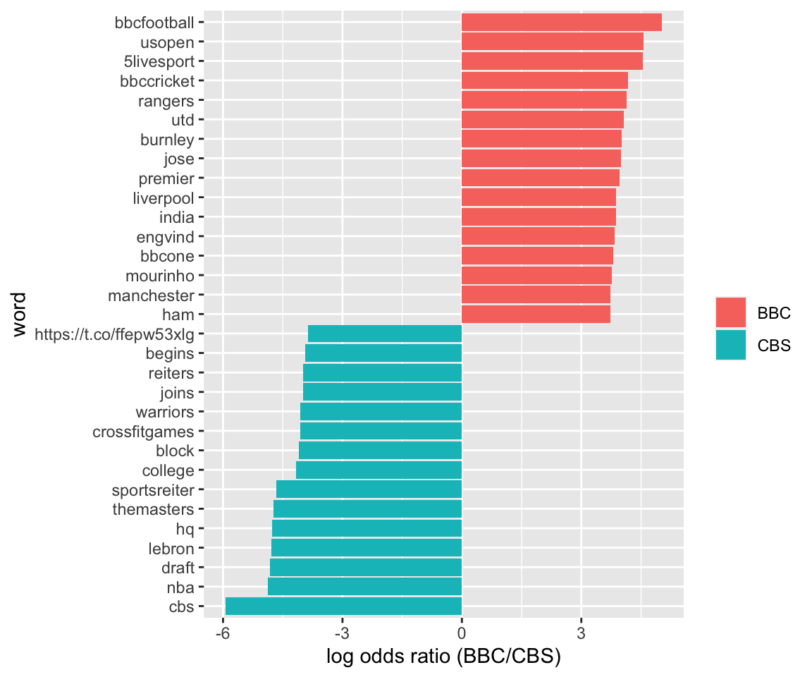
##Frequencies of key words
Here, I have chosen a list of seven “key words” - that is, seven sports that are played in the US and UK. I filtered the list of frequencies for each word to only look for these words. Note that there are a few words that do not show up for a couple of the user names. Because these don’t show up, if we leave them out, the bar plot looks a bit weird.
#IF there are 0s, they won't show up in the bar plot
sportslist = c("football", "soccer", "baseball", "basketball", "tennis", "rugby", "cricket")

frequentsports = timelines_frequency %>% filter(word %in% sportslist)

dim(frequentsports)
## [1] 18 5ggplot(frequentsports, aes(x = word, fill = screen_name)) + geom_bar(aes(weight = n), position = "dodge")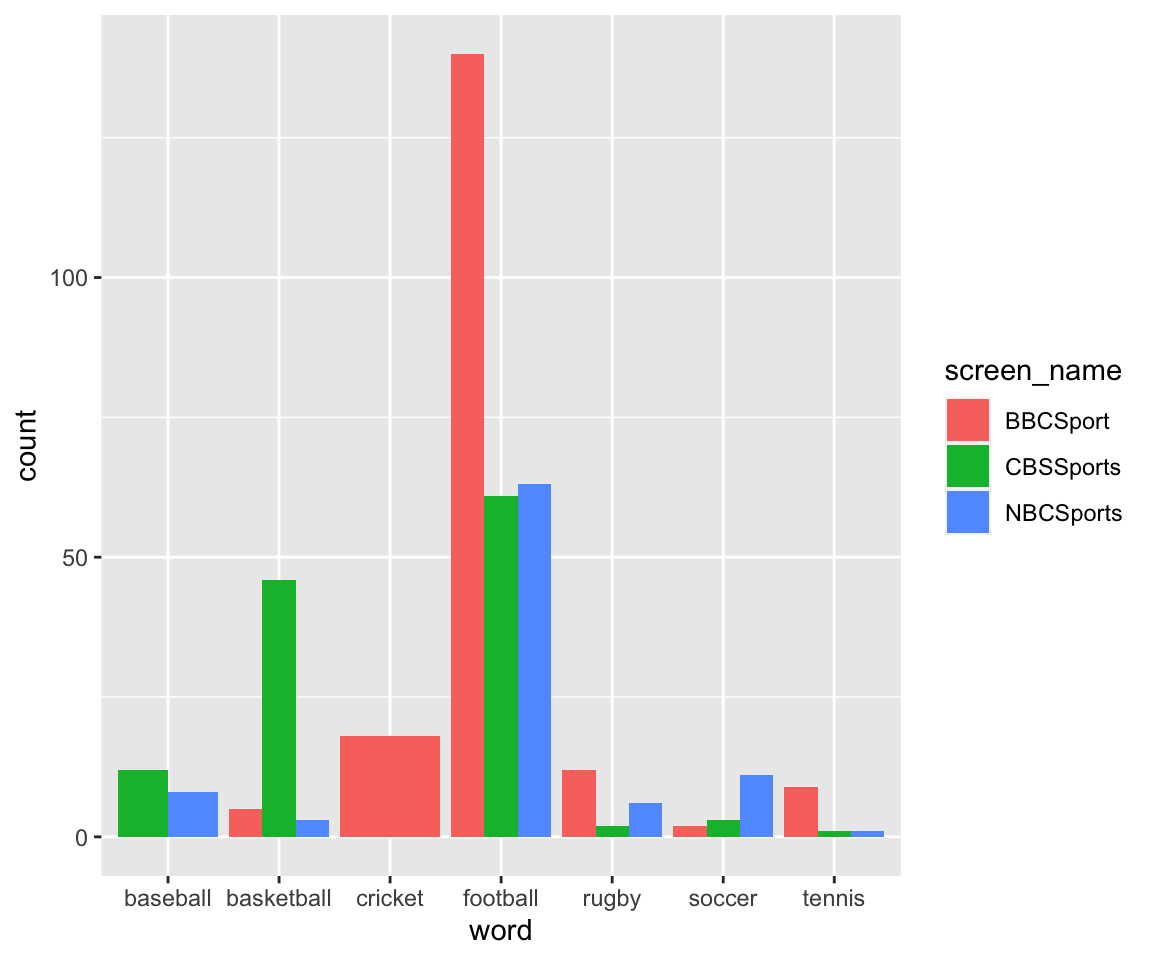
If we want to include these specifically in the bar plot, even with values of 0, we need to make a new grid with all possible combinations of user_name and sport, and then merge this with the frequencies given from the tweets. Any word*screen_name pairs that do not exist will be filled in with a 0. This gives the bar plot we are looking for!
#creating a full data grid with zeros to preserve shape of bar plot

sportslist = data.frame(word = rep(c("football", "soccer", "baseball", "basketball", "tennis", "rugby", "cricket"), 3), screen_name = rep(c("BBCSport", "NBCSports", "CBSSports"), each = 7))

frequentsports = timelines_frequency %>% filter(word %in% sportslist$word)

fullsports_timelines = full_join(frequentsports, sportslist, by = c("screen_name", "word"), fill = 0)  %>% replace(., is.na(.), 0)


ggplot(fullsports_timelines, aes(x = word, fill = screen_name)) + geom_bar(aes(weight = n), position = "dodge")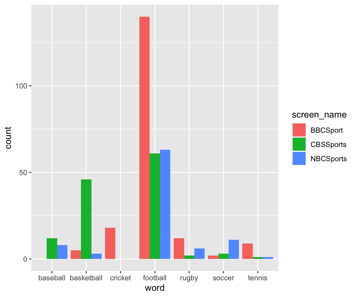
##Sentiment analysis In order to do sentiment analysis, we will use a few datasets from R’s tidytext package: the sentiments dataset, and the stop_words dataset, which comes with three general-purpose lexicons:
- FINN from Finn Årup Nielsen,
- bing from Bing Liu and collaborators, and
- nrc from Saif Mohammad and Peter Turney.
From the Text Mining with R book (Section 2.1):
All three of these lexicons are based on unigrams, i.e., single words. These lexicons contain many English words and the words are assigned scores for positive/negative sentiment, and also possibly emotions like joy, anger, sadness, and so forth. The nrc lexicon categorizes words in a binary fashion (“yes”/“no”) into categories of positive, negative, anger, anticipation, disgust, fear, joy, sadness, surprise, and trust. The bing lexicon categorizes words in a binary fashion into positive and negative categories. The AFINN lexicon assigns words with a score that runs between -5 and 5, with negative scores indicating negative sentiment and positive scores indicating positive sentiment. All of this information is tabulated in the sentiments dataset, and tidytext provides a function get_sentiments() to get specific sentiment lexicons without the columns that are not used in that lexicon.
For the bing lexicon, a sentiment score is given by the number of times a word shows up in the corpus. We calculate sentiment = positive - negative, so that negative words have a negative score, and positive words have a positive score. We choose the top 30 words in terms of sentiment scores - that is, the 30 most frequent words that are related to sentiment.
data("sentiments")

sports_sentiments_bing <- timelines_frequency %>%
  inner_join(get_sentiments("bing")) %>%
  spread(sentiment, n,fill = 0) %>%
  mutate(sentiment = positive - negative) %>%
  top_n(30, abs(sentiment))
## Joining, by = "word"head(sports_sentiments_bing)## # A tibble: 6 x 7
## # Groups: screen_name [1]
## screen_name word total freq negative positive sentiment
## <chr> <chr> <int> <dbl> <dbl> <dbl> <dbl>
## 1 BBCSport bad 27662 0.000542 15 0 -15
## 2 BBCSport break 27662 0.000868 24 0 -24
## 3 BBCSport brilliant 27662 0.000398 0 11 11
## 4 BBCSport champion 27662 0.000651 0 18 18
## 5 BBCSport defeat 27662 0.00119 0 33 33
## 6 BBCSport defender 27662 0.000615 0 17 17ggplot(sports_sentiments_bing, aes(word, sentiment, fill = sentiment<0)) + geom_col(show.legend = FALSE) +coord_flip()+ facet_wrap(~screen_name, ncol = 3, scales = "free_x")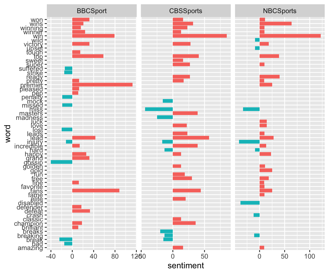
For the afinn sentiment dataset, we calculate sentiment by multiplying the score given by the dataset (ranging form -5 to 5) by the number of instances of that word. Once again, the top 30 words are chosen.
sports_sentiments_afinn <- timelines_frequency %>%
  inner_join(tidytext::get_sentiments("afinn")) %>% mutate(sentiment = n*value) %>%
  top_n(30, abs(sentiment))
## Joining, by = "word"head(sports_sentiments_afinn)## # A tibble: 6 x 7
## # Groups: screen_name [3]
## screen_name word n total freq value sentiment
## <chr> <chr> <int> <int> <dbl> <dbl> <dbl>
## 1 NBCSports win 122 27818 0.00439 4 488
## 2 CBSSports win 85 26080 0.00326 4 340
## 3 BBCSport win 79 27662 0.00286 4 316
## 4 NBCSports wins 64 27818 0.00230 4 256
## 5 BBCSport top 58 27662 0.00210 2 116
## 6 CBSSports block 54 26080 0.00207 -1 -54ggplot(sports_sentiments_afinn, aes(word, sentiment, fill = sentiment<0)) + geom_col(show.legend = FALSE) +coord_flip()+ facet_wrap(~screen_name, ncol = 3, scales = "free_x")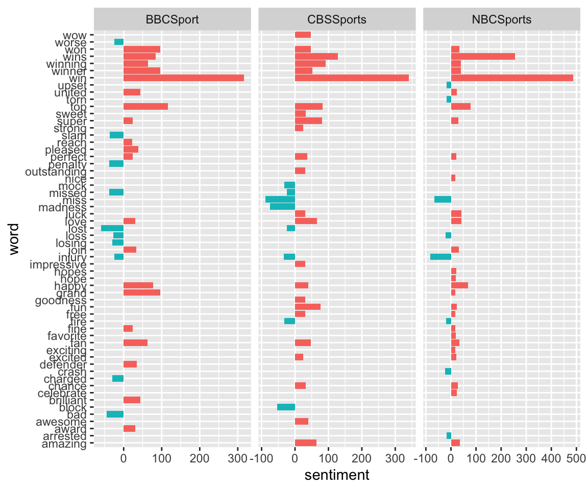
Here, we want to compare the counts per screen name for each sentiment word. The top 30 most frequent sentiment words, regardless of their positivity/negativity, are chosen.
bing_word_counts =  timelines_tidy_tweets %>% inner_join(get_sentiments("bing")) %>%
  count(screen_name, word, sentiment, sort = TRUE) %>%  ungroup()
## Joining, by = "word"head(bing_word_counts)## # A tibble: 6 x 4
## screen_name word sentiment n
## <chr> <chr> <chr> <int>
## 1 NBCSports win positive 122
## 2 BBCSport premier positive 113
## 3 BBCSport fans positive 88
## 4 CBSSports win positive 85
## 5 BBCSport win positive 79
## 6 NBCSports wins positive 64bing_word_counts %>%
group_by(screen_name, sentiment) %>%
top_n(30) %>%
ungroup() %>%
mutate(word = reorder(word, n)) %>%
ggplot(aes(word, n, fill = screen_name)) +
geom_col(show.legend = FALSE) +
facet_wrap(~sentiment, scales = "free_y") +
labs(y = "Contribution to sentiment",
x = NULL) +
coord_flip()## Selecting by n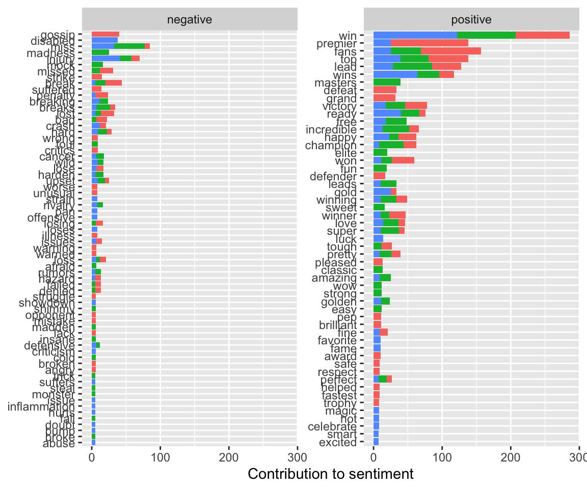
And finally, we can create a word cloud using the top 100 words from the dataset.
timelines_tidy_tweets %>%
  anti_join(stop_words) %>%
  group_by(screen_name) %>%
  count(word) %>%
  with(wordcloud(word, n, max.words = 100))
## Joining, by = "word"## Warning in wordcloud(word, n, max.words = 100): england could not be fit on
## page. It will not be plotted.## Warning in wordcloud(word, n, max.words = 100): stream could not be fit on page.
## It will not be plotted.## Warning in wordcloud(word, n, max.words = 100): championship could not be fit on
## page. It will not be plotted.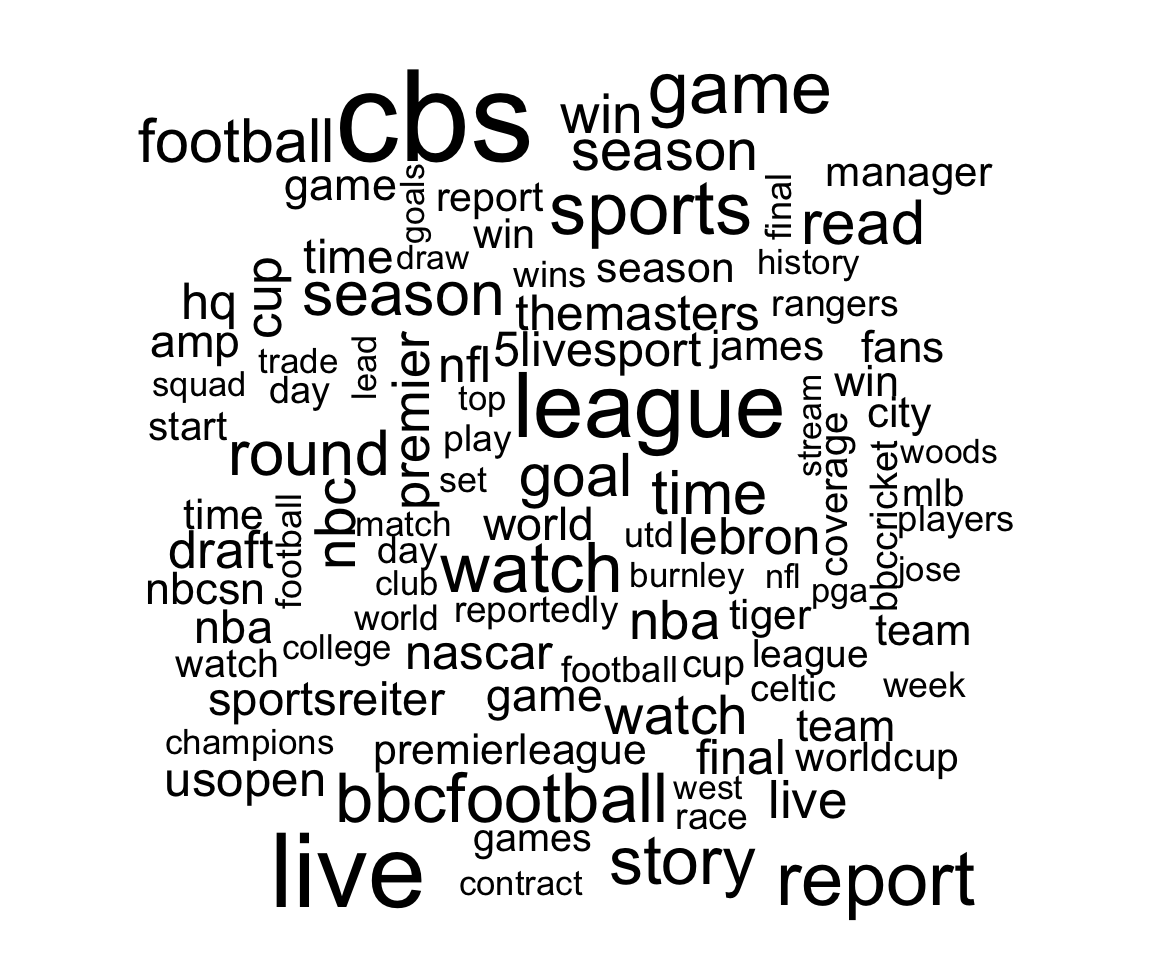
#Comparing tweets with certain search terms ##Processing data Now we will go on to searching for tweets that have certain words included. Once again, I processed the data to get rid of the extraneous information.
footballterms_processed = footballterms %>% select(screen_name, created_at, text, is_retweet, is_quote, favorite_count, retweet_count, hashtags, lat, lng)##Locations and time series What if we want to see where/when tweets are being produced? I used previously the lat_lng() function from the rtweet package. This converts the geocoded information that is buried in the huge dataset into latitude and longitude. Note that I didn’t search specifically for geotagged tweets, so only a subset of my tweets have latitudes and longitudes. If you want to search for geotagged tweets, you can give search_tweets() a latitude, longitude and radius to geographically bound your search results, as such:
#not run
rt <- search_tweets("rstats", n = 500, include_rts = FALSE, geocode = "37.78,-122.40,1mi")
Here, I am first filtering my data so that I only include data with values for latitude and longitude. (I am filtering only on latitude, with the presumption that if I have a value for latitude, I will have one for longitude as well.)
I then am looking up the geocode for the United States, and calling to get a map from google maps. This is the basis of my geographical plot. The function get_map and the plotting function ggmap are found in the ggmap package. This allows you to use the map as a base for a ggplot-type figure, as I do below.
head(footballterms_processed)## # A tibble: 6 x 10
## screen_name created_at text is_retweet is_quote favorite_count
## <chr> <dttm> <chr> <lgl> <lgl> <int>
## 1 RampartapD 2018-09-05 14:22:19 "Jus… TRUE FALSE 0
## 2 TDMindsTA 2018-09-05 14:22:19 "@de… FALSE FALSE 0
## 3 leahcimekim 2018-09-05 14:22:19 "@Br… FALSE FALSE 0
## 4 leahcimekim 2018-09-05 14:14:16 "@Br… FALSE FALSE 0
## 5 leahcimekim 2018-09-05 14:13:50 "@Br… FALSE FALSE 0
## 6 D_Valladar… 2018-09-05 14:22:19 "4 D… TRUE FALSE 0
## # … with 4 more variables: retweet_count <int>, hashtags <list>, lat <dbl>,
## # lng <dbl>dim(footballterms_processed[!is.na(footballterms_processed$lat),])## [1] 1075 10footballgeo = footballterms_processed %>% filter(!is.na(lat))
UScode = geocode("United States")## Source : https://maps.googleapis.com/maps/api/geocode/json?address=United+States&key=xxxusmap<-get_map(location=UScode, zoom=4, maptype = "terrain", source = "google")## Source : https://maps.googleapis.com/maps/api/staticmap?center=37.09024,-95.712891&zoom=4&size=640x640&scale=2&maptype=terrain&language=en-EN&key=xxxggmap(usmap) + geom_point(data = footballgeo, aes(x = lng, y = lat, color = is_retweet))## Warning: Removed 1 rows containing missing values (geom_point).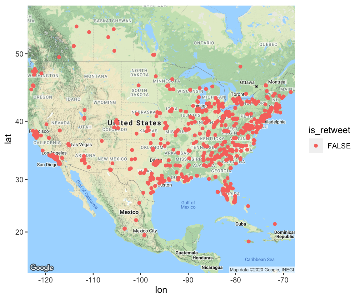
Here’s another example of processing and tokenizing tweets. I am doing the same thing I did before for the timelines data - processing the strings, then getting frequencies.
Note that I am stripping the date and time from the created_at variable. The created_at variable is in a special date-time format for R, which makes plotting time series data very easy, so I don’t recommend you necessarily use the stripped data to create plots.
data("stop_words")

remove_reg <- "@|&|#"
football_tweets <- footballterms_processed %>%
  filter(is_retweet == FALSE) %>%
  mutate(text = str_remove_all(text, remove_reg)) %>%
  unnest_tokens(word, text, token = "tweets") %>%
  filter(!word %in% stop_words$word,
         !word %in% str_remove_all(stop_words$word, "'"),
         str_detect(word, "[a-z]"),
         !str_detect(word, "^http"),
         !word=="amp")
## Using `to_lower = TRUE` with `token = 'tweets'` may not preserve URLs.head(football_tweets)## # A tibble: 6 x 10
## screen_name created_at is_retweet is_quote favorite_count
## <chr> <dttm> <lgl> <lgl> <int>
## 1 TDMindsTA 2018-09-05 14:22:19 FALSE FALSE 0
## 2 TDMindsTA 2018-09-05 14:22:19 FALSE FALSE 0
## 3 TDMindsTA 2018-09-05 14:22:19 FALSE FALSE 0
## 4 TDMindsTA 2018-09-05 14:22:19 FALSE FALSE 0
## 5 TDMindsTA 2018-09-05 14:22:19 FALSE FALSE 0
## 6 TDMindsTA 2018-09-05 14:22:19 FALSE FALSE 0
## # … with 5 more variables: retweet_count <int>, hashtags <list>, lat <dbl>,
## # lng <dbl>, word <chr>football_frequency <- football_tweets %>%
# group_by(screen_name) %>%
count(word, sort = TRUE) %>%
left_join(football_tweets) %>%
rename(number = n) %>%
mutate(freq = number/n(), date = strftime(created_at, format = "%m/%d/%y"), time = strftime(created_at, format="%H:%M:%S")) %>% select(screen_name, created_at, word, number, freq, everything()) %>% select(-hashtags) ## Joining, by = "word"Here, I am plotting the top 20 most frequent words.
football_frequency %>% group_by(word) %>% summarise(number = max(number)) %>% arrange(desc(number)) %>% top_n(20, number) %>% ggplot(aes(reorder(word, number), number)) +geom_col() +coord_flip()## `summarise()` ungrouping output (override with `.groups` argument)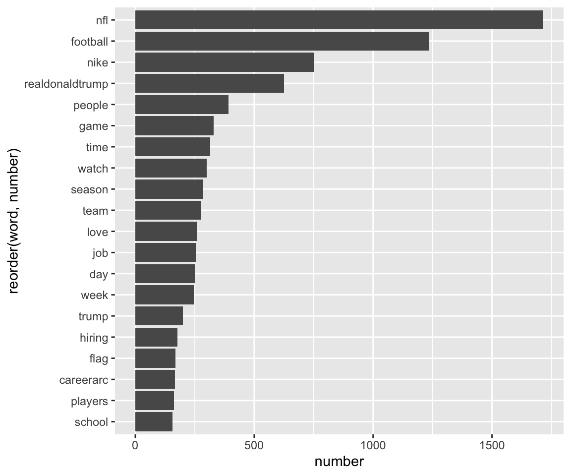
And here, I am doing a time-series plot using the ts_plot function from the rtweet package. First, I am looking at the data by hour, and then by minute. Because I collected this data from a small window of time, these aren’t particularly informative, but if you had a larger dataset, you could do some cool time series work. Tidy Text Mining with R gives another example of time-dynamic analyses.
football10 = football_frequency %>% group_by(word) %>% summarise(number = max(number)) %>% arrange(desc(number))%>%top_n(10,number)%>% left_join(football_frequency) %>% group_by(word)## `summarise()` ungrouping output (override with `.groups` argument)## Joining, by = c("word", "number")ts_plot(football10, "hours")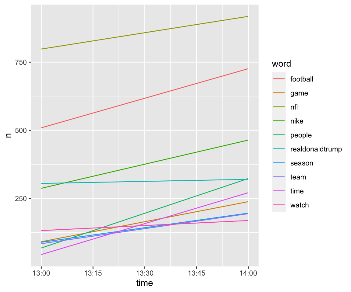
ts_plot(football10, "mins")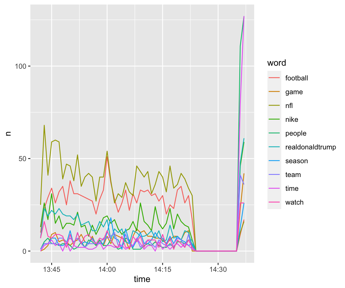
And finally, you can create another word cloud!
football_frequency %>%
  anti_join(stop_words)%>%
  group_by(word) %>% summarise(number = max(number)) %>% top_n(100, number)%>%
  with(wordcloud(word, number, max.words = 100))
## Joining, by = "word"## `summarise()` ungrouping output (override with `.groups` argument)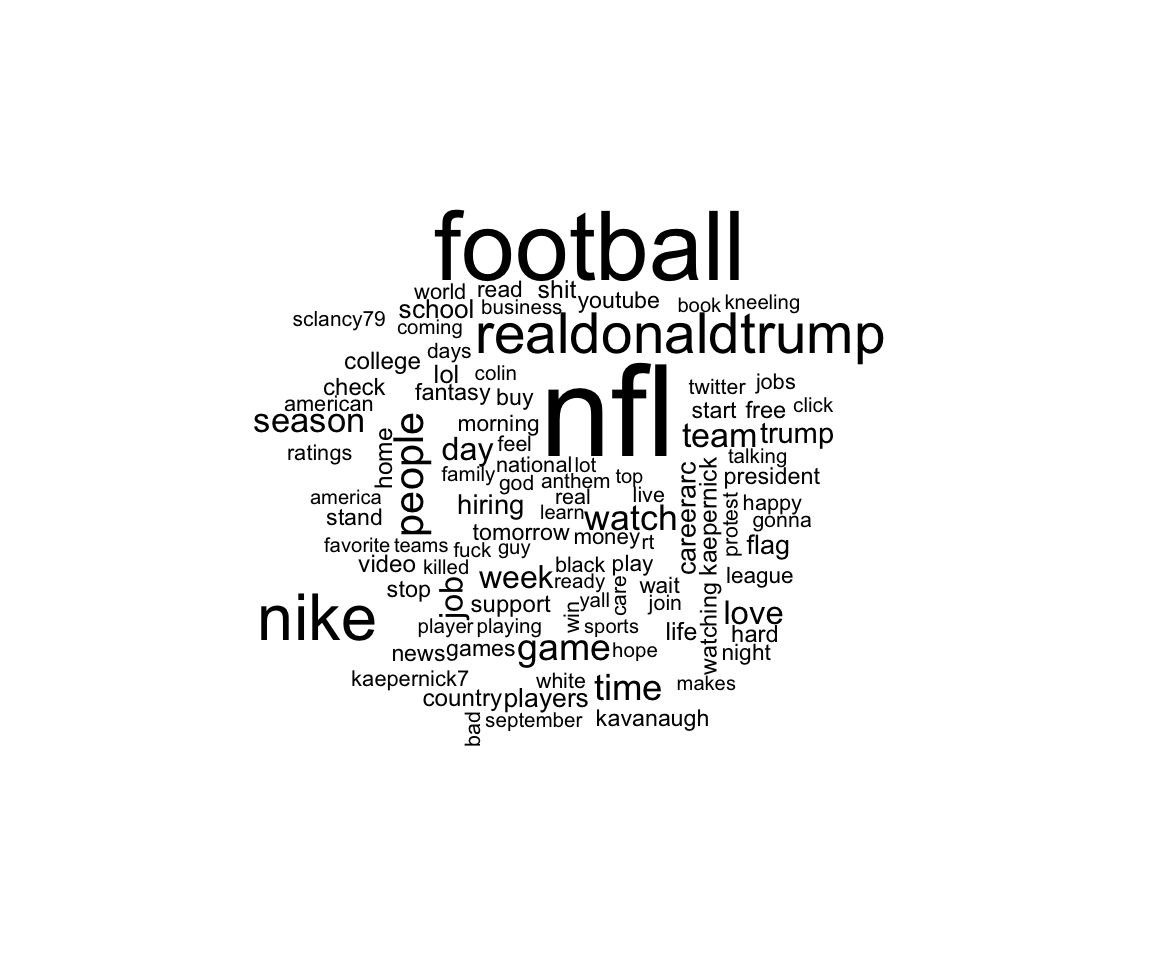
#Another example of multiple search terms
Finally, I am looking at the relative distributions of dogs, cats and hamsters on Twitter. Note that I created a variable a while ago on my dataset, called animalmentioned, which pulled out which of my three search terms is mentioned in the tweet. I created the tokenized tweets file one more. ##Data processing
animals_processed = cuteanimals %>% select(screen_name, animalmentioned, created_at, text, is_retweet, is_quote, favorite_count, retweet_count, hashtags, lat, lng)

head(animals_processed)
## # A tibble: 6 x 11
## screen_name animalmentioned created_at text is_retweet is_quote
## <chr> <chr> <dttm> <chr> <lgl> <lgl>
## 1 denisngahu cat 2018-09-05 17:07:18 "Rem… TRUE FALSE
## 2 AnimalAnge… cat 2018-09-05 17:07:18 "Ple… TRUE FALSE
## 3 pecanacres <NA> 2018-09-05 17:07:15 "Fev… FALSE FALSE
## 4 RufnekBob dog 2018-09-05 17:07:15 "Dog… TRUE FALSE
## 5 JesionekSa… cat 2018-09-05 17:07:15 "@Je… FALSE FALSE
## 6 badgaIzak cat 2018-09-05 17:07:13 "I j… TRUE FALSE
## # … with 5 more variables: favorite_count <int>, retweet_count <int>,
## # hashtags <list>, lat <dbl>, lng <dbl> remove_reg <- "@|&|#"
animal_tweets <- animals_processed %>%
filter(is_retweet == FALSE) %>%
mutate(text = str_remove_all(text, remove_reg)) %>%
unnest_tokens(word, text, token = "tweets") %>%
filter(!word %in% stop_words$word,
!word %in% str_remove_all(stop_words$word, "'"),
str_detect(word, "[a-z]"),
!str_detect(word, "^http"),
!word =="amp")## Using `to_lower = TRUE` with `token = 'tweets'` may not preserve URLs.##Time and Space Here, I am looking at tweets over time and space by the animal mentioned. As you can see, not a lot of people are talking about hamsters!
animalgeo = animals_processed %>% filter(!is.na(lat), !is.na(animalmentioned))
ggmap(usmap) + geom_point(data = animalgeo, aes(x = lng, y = lat, color = animalmentioned))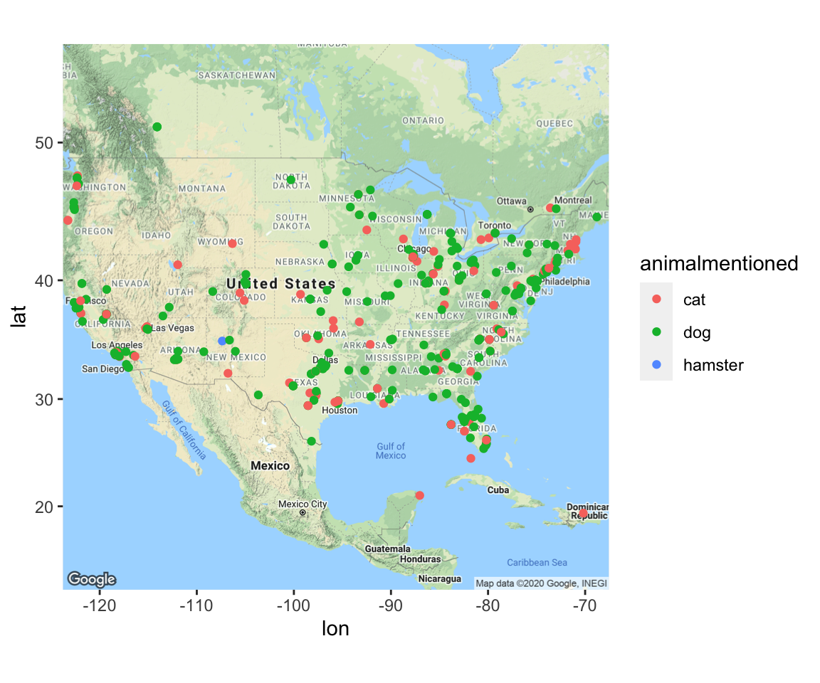
Here, I am comparing the top 10 words used in reference to animals.
animal_frequency <- animal_tweets %>%
#  group_by(screen_name) %>%
  count(word, sort = TRUE) %>%
  left_join(animal_tweets) %>%
  rename(number = n) %>%
  mutate(freq = number/n(), date = strftime(created_at, format = "%m/%d/%y"), time = strftime(created_at, format="%H:%M:%S")) %>% select(screen_name, created_at, word, number, freq, everything()) %>% select(-hashtags)
## Joining, by = "word"animal10 = animal_frequency %>% group_by(word) %>% summarise(number = max(number)) %>% arrange(desc(number))%>%top_n(10,number)%>% left_join(animal_frequency) %>% group_by(word)## `summarise()` ungrouping output (override with `.groups` argument)## Joining, by = c("word", "number")ts_plot(animal10, "hours")
ts_plot(animal10, "mins")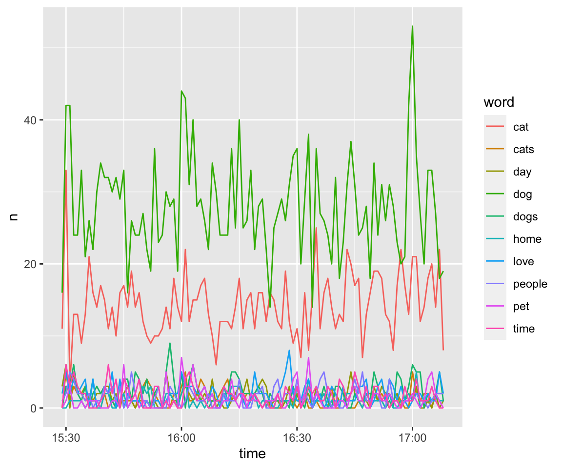
##Sentiments Let’s look at sentiments in reference to animals. Once again I will use the Bing sentiment corpus. I also have created another dataset, animals_bing_time, that looks at sentiments over time by dividing the timestamps into 40 windows.
data("sentiments")

animals_bing <- animal_tweets %>%
  inner_join(get_sentiments("bing"))%>%
  count(word, sentiment, animalmentioned, sort = TRUE) %>%
  spread(sentiment, n,fill = 0)%>%
  mutate(sentiment = positive - negative) %>%
  top_n(30, abs(sentiment))
## Joining, by = "word"animals_bing_time <- animal_tweets %>%
inner_join(get_sentiments("bing"))%>%
count(index = as.numeric(cut(created_at, 40)), sentiment, sort = TRUE) %>%
spread(sentiment, n,fill = 0)%>%
mutate(sentiment = positive - negative)## Joining, by = "word"ggplot(animals_bing, aes(word, sentiment, fill = sentiment<0)) +
geom_col(show.legend = FALSE) +coord_flip()+
facet_wrap(~animalmentioned, ncol = 3, scales = "free_x")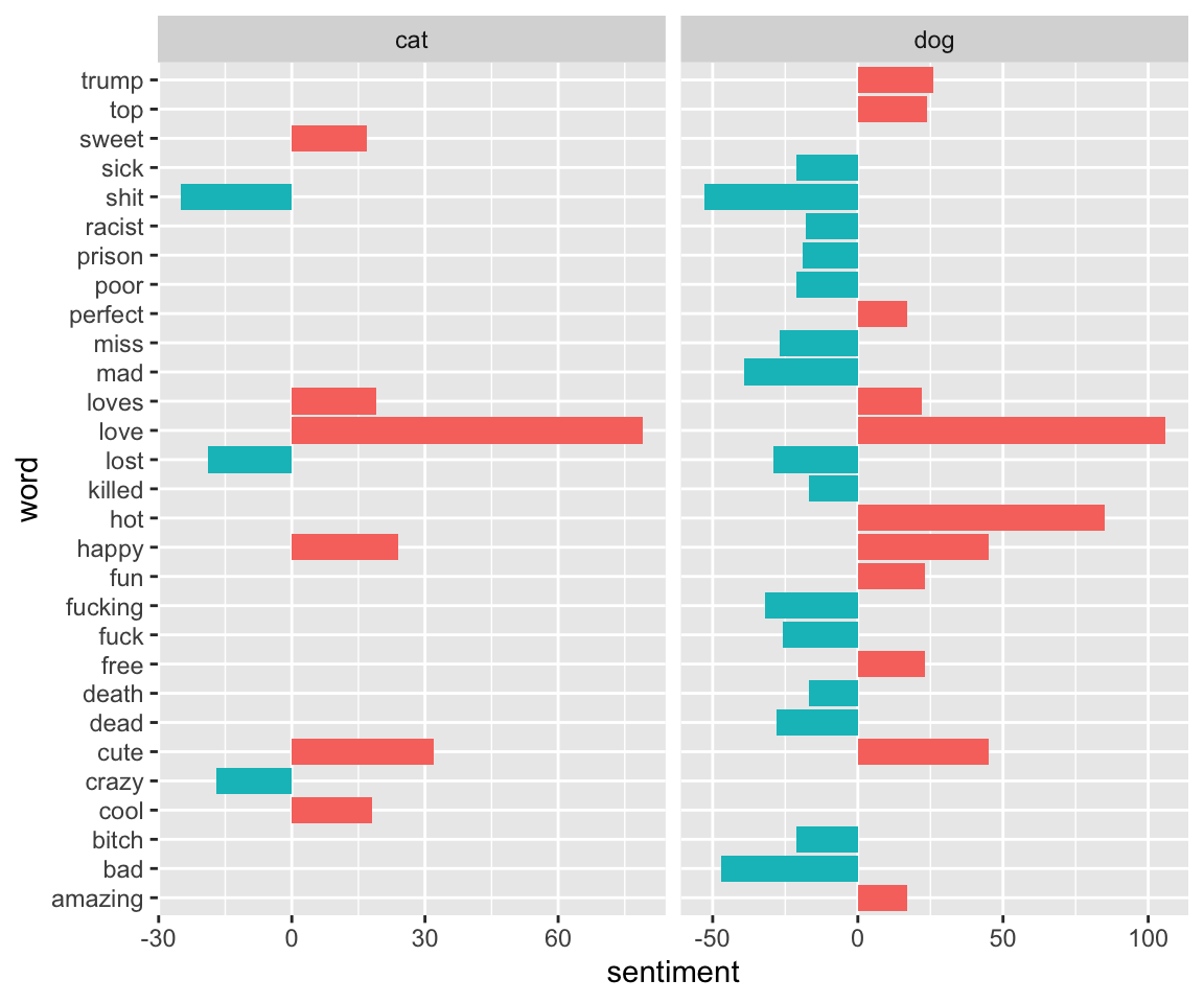
ggplot(animals_bing_time, aes(index, sentiment, fill = sentiment<0)) +
  geom_col(show.legend = FALSE) + scale_x_continuous(breaks=seq(0,40,10))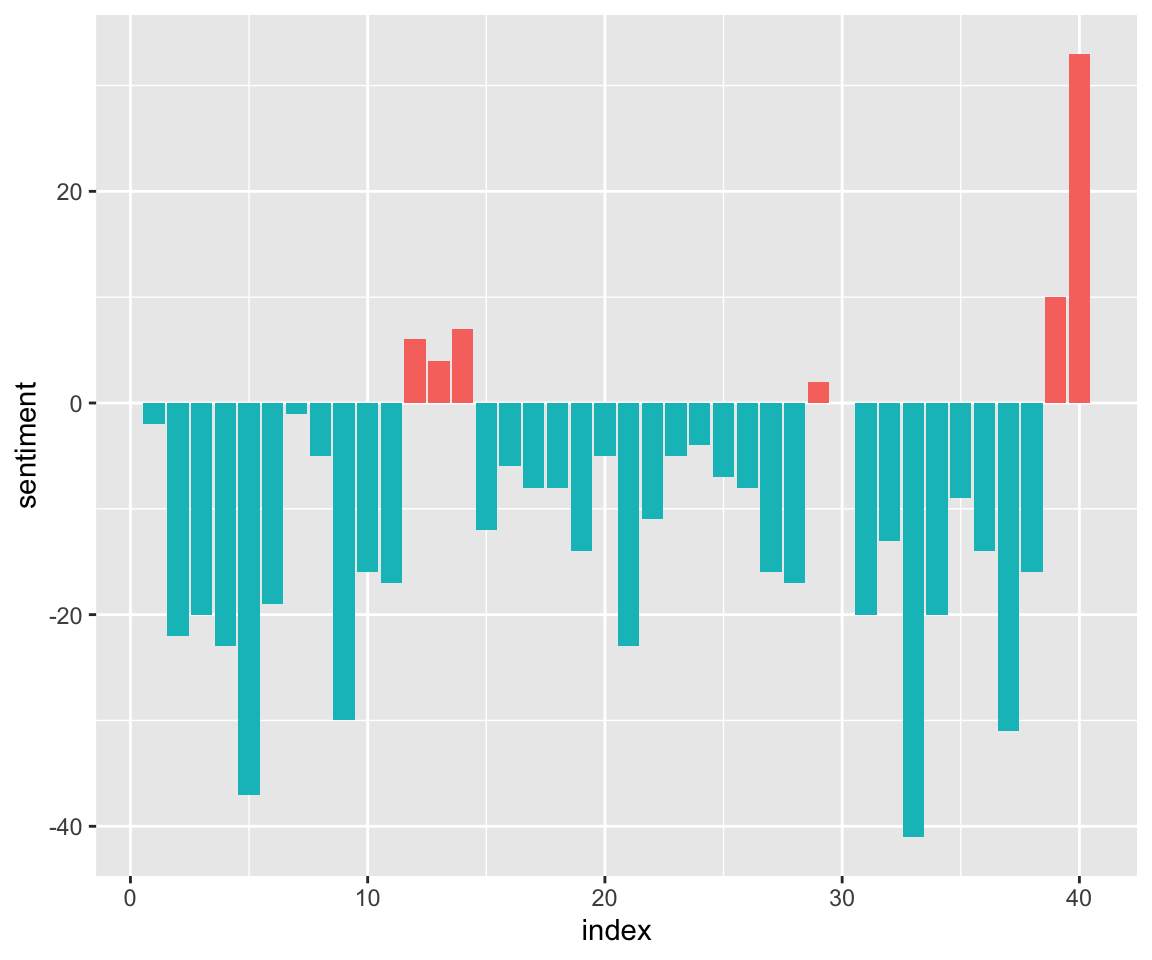
animals_bing_time %>% top_n(50, abs(sentiment)) %>%ggplot(aes(index, sentiment, fill = sentiment<0)) + geom_col(show.legend = FALSE) + scale_x_continuous(breaks=seq(0,40,10))
Again, I am using the afinn sentiment corpus.
animals_sentiments_afinn <- animal_frequency %>%
  inner_join(get_sentiments("afinn")) %>% mutate(sentiment = number*value, index = as.numeric(cut(created_at, 40))) %>%count(word, sentiment, sort = TRUE)
## Joining, by = "word"animals_sentiments_afinn %>% top_n(10) %>%
ggplot( aes(reorder(word, desc(sentiment)), sentiment, fill = sentiment<0)) +
geom_col(show.legend = FALSE) +coord_flip() + xlab("Word")## Selecting by n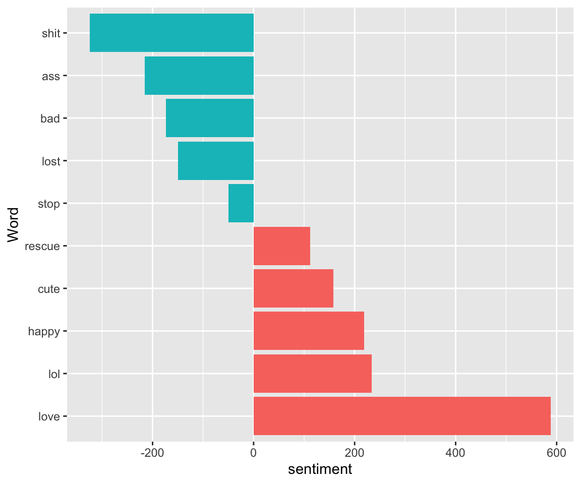
animals_counts_nbing =  animal_tweets %>% inner_join(get_sentiments("bing")) %>%
  count(animalmentioned, word, sentiment, sort = TRUE) %>%
  ungroup()
## Joining, by = "word"head(animals_counts_nbing)## # A tibble: 6 x 4
## animalmentioned word sentiment n
## <chr> <chr> <chr> <int>
## 1 dog love positive 106
## 2 dog hot positive 85
## 3 cat love positive 79
## 4 dog shit negative 53
## 5 dog bad negative 47
## 6 dog cute positive 45animals_counts_nbing %>%
group_by(animalmentioned, sentiment) %>%
top_n(10) %>%
ungroup() %>%
mutate(word = reorder(word, n)) %>%
ggplot(aes(word, n, fill = animalmentioned)) +
geom_col(show.legend = FALSE) +
facet_wrap(~sentiment, scales = "free_y") +
labs(y = "Contribution to sentiment",
x = NULL) +
coord_flip()## Selecting by n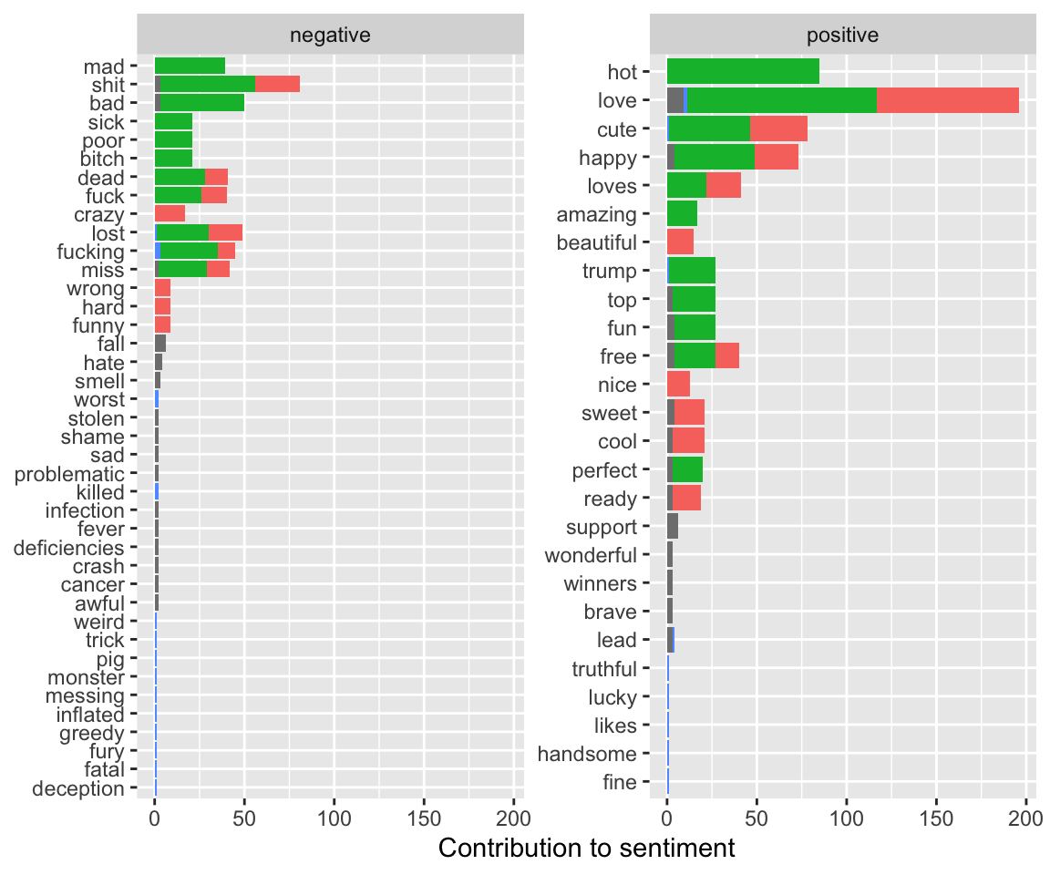 And a word cloud!
animal_tweets %>%
  anti_join(stop_words) %>%
  count(word) %>%
  with(wordcloud(word, n, max.words = 100))
## Joining, by = "word"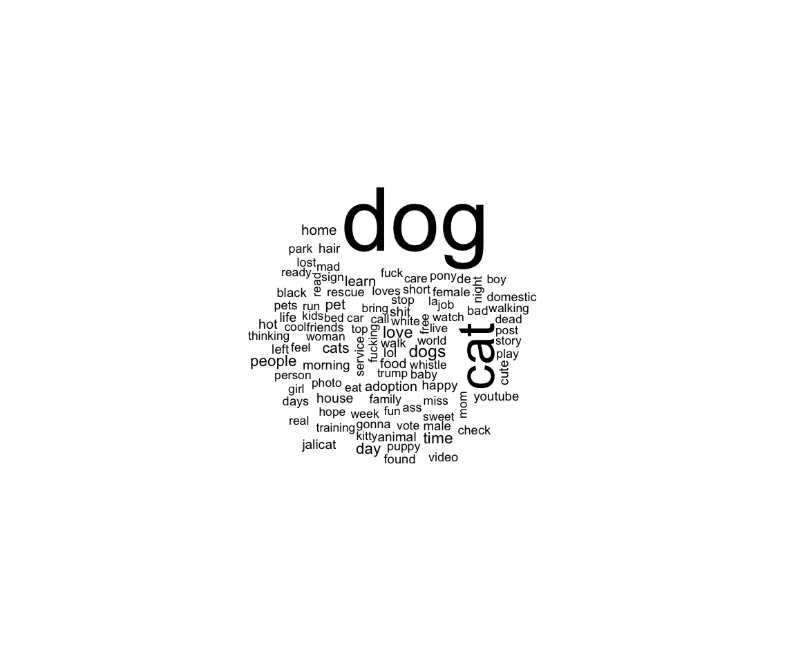
#A few final words
Using the other packages I mentioned, as well as rtweet, you can do a lot - you can stream tweets, follow users, etc. Here, I used a bounding box I determined interactively here to stream tweets found in Chicago. (I tried Champaign, but we don’t seem to tweet much!)
champaignbox = c(-88.290213,40.06123,-88.178074,40.166118)
chicagobox = c(-87.741984,41.790998,-87.528422,41.989486)
filterStream( file="tweets_rstats.json", locations=chicagobox, timeout=60, oauth=my_oauth )
tweets.df <- parseTweets("tweets_rstats.json")