R Modeling Workshop
The aim of this workshop is to teach you the basics of statistical models in R.
The materials for this workshop can be found here.
What is the point?
When looking at data, we want to determine if there is a relationship between our independent and dependent variables. A traditional method of analysis in Linguistics and associated fields is regression analysis, which helps understand how a particular variable (the dependent variable) changes when other variables (independent variables, or predictors) are varied.
When running regression analyses, the dependent variable must be continuous. The independent variables can be continuous, discrete, or categorical.
When we run regression analyses on our data, we first need to make sure a few basic assumptions are met:
- The sample is representative of the population.
- The predictors are measured with no error.
- The predictors are linearly independent, i.e. it is not possible to express any predictor as a linear combination of the others.
We will go through further assumptions as we go through the workshop.
Data
The data I will be using during this tutorial is from the University of Wisconsin’s X-Ray Microbeam Speech Production Database. The database has the following variables:
- v = vowel
- f0
- f1-f4
- ulx and uly = x and y coordinates of the upper lip
- llx and lly = x and y coordinates of the lower lip
- t(1-4)x and t(1-4)y = x and y coordinates of the tongue at position (1-4)
- mnix and mniy = x and y coordinates of the mandibular incisor
- mnmx and mnmy = x and y coordinates of the mandibular molar
ubdb = read.csv("ubdb.csv", header = T)
head(ubdb)
## v f0 f1 f2 f3 f4 ulx uly llx lly t1x
## 1 AA 117.9440 685.407 1197.050 2191.48 3336.96 13932 18276 6539 -30434 -23064
## 2 IH 112.8280 418.372 985.526 2487.43 3011.10 20501 20067 5382 -22754 -19155
## 3 AO 93.0954 590.657 972.832 2020.60 2789.85 19325 19404 13488 -16881 -27701
## 4 EH 102.2070 614.993 1477.480 2312.54 3231.13 14055 18779 8355 -31634 -13440
## 5 AO 95.1051 560.905 1071.830 1815.31 2777.59 19559 21403 13222 -17716 -23812
## 6 IH 100.8450 201.074 1246.360 2390.22 3494.73 13907 16145 10587 -16234 -19836
## t1y t2x t2y t3x t3y t4x t4y mnix mniy mnmx mnmy
## 1 -4335 -35728 -255 -46156 6775 -57700 13213 -1210 -12864 -42867 -8388
## 2 5498 -30598 10135 -41026 14935 -55410 17009 -1726 -6362 -44347 -3640
## 3 85 -36820 10226 -46626 17044 -60265 18089 -646 -11293 -42029 -7787
## 4 -8626 -25020 -878 -35575 6039 -48541 7436 953 -16019 -40606 -10839
## 5 3805 -32471 12748 -42574 18192 -56299 15808 191 -11150 -41519 -7347
## 6 4807 -29710 11789 -40145 17257 -55107 14865 -1886 -7813 -44639 -4746summary(ubdb)## v f0 f1 f2
## Length:1073 Min. : 0.00 Min. : 89.3 Min. : 684.9
## Class :character 1st Qu.: 89.19 1st Qu.: 291.2 1st Qu.:1220.0
## Mode :character Median : 96.81 Median : 430.1 Median :1484.1
## Mean : 94.07 Mean : 437.4 Mean :1497.9
## 3rd Qu.:103.18 3rd Qu.: 564.2 3rd Qu.:1758.3
## Max. :137.50 Max. :1284.5 Max. :2572.6
## f3 f4 ulx uly llx
## Min. :1368 Min. :2297 Min. :11793 Min. :11444 Min. : 461
## 1st Qu.:2188 1st Qu.:3093 1st Qu.:14134 1st Qu.:17027 1st Qu.: 7249
## Median :2352 Median :3383 Median :14976 Median :18033 Median : 8931
## Mean :2375 Mean :3397 Mean :15366 Mean :17877 Mean : 9000
## 3rd Qu.:2525 3rd Qu.:3652 3rd Qu.:16201 3rd Qu.:18825 3rd Qu.:10810
## Max. :3837 Max. :4689 Max. :21092 Max. :23841 Max. :17787
## lly t1x t1y t2x
## Min. :-35268 Min. :-36533 Min. :-14089.0 Min. :-43405
## 1st Qu.:-24962 1st Qu.:-19836 1st Qu.: -3307.0 1st Qu.:-31378
## Median :-22224 Median :-15257 Median : -54.0 Median :-26343
## Mean :-22393 Mean :-16737 Mean : -218.9 Mean :-27558
## 3rd Qu.:-19517 3rd Qu.:-12428 3rd Qu.: 3389.0 3rd Qu.:-23596
## Max. :-11031 Max. : -5494 Max. : 14836.0 Max. :-16923
## t2y t3x t3y t4x
## Min. :-7592 Min. :-52913 Min. : 1051 Min. :-66180
## 1st Qu.: 4132 1st Qu.:-42054 1st Qu.:11226 1st Qu.:-55572
## Median : 8426 Median :-37292 Median :16017 Median :-51926
## Mean : 7863 Mean :-38021 Mean :15338 Mean :-52621
## 3rd Qu.:11900 3rd Qu.:-34018 3rd Qu.:20273 3rd Qu.:-49451
## Max. :19404 Max. :-27306 Max. :24056 Max. :-43324
## t4y mnix mniy mnmx
## Min. : 7436 Min. :-4160 Min. :-19839 Min. :-47257
## 1st Qu.:15148 1st Qu.:-1674 1st Qu.: -9919 1st Qu.:-44127
## Median :18906 Median :-1081 Median : -7640 Median :-43396
## Mean :18747 Mean :-1033 Mean : -8321 Mean :-43309
## 3rd Qu.:22853 3rd Qu.: -467 3rd Qu.: -6055 3rd Qu.:-42593
## Max. :25995 Max. : 3410 Max. : -3140 Max. :-38797
## mnmy
## Min. :-12229
## 1st Qu.: -4419
## Median : -2558
## Mean : -3030
## 3rd Qu.: -1300
## Max. : 1029Simple linear regression
Let’s say we want to determine if there is a predictable relationship between articulation and acoustics. Let’s see if there is a relationship between tongue height and the first formant. The first thing we want to do is examine the data.
plot(ubdb$t1y, ubdb$f1)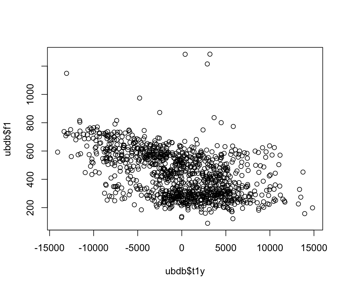
It looks like the relationship is linear (specifically, of the form y=mx+b+e) based on a first glance at the data. We can model the relationship between these two variables using the lm() function.
lm1 = lm(f1~t1y, data = ubdb)
summary(lm1)
##
## Call:
## lm(formula = f1 ~ t1y, data = ubdb)
##
## Residuals:
## Min 1Q Median 3Q Max
## -320.84 -112.21 1.22 102.13 900.21
##
## Coefficients:
## Estimate Std. Error t value Pr(>|t|)
## (Intercept) 4.340e+02 4.373e+00 99.25 <2e-16 ***
## t1y -1.557e-02 8.544e-04 -18.23 <2e-16 ***
## ---
## Signif. codes: 0 '***' 0.001 '**' 0.01 '*' 0.05 '.' 0.1 ' ' 1
##
## Residual standard error: 143.1 on 1071 degrees of freedom
## Multiple R-squared: 0.2367, Adjusted R-squared: 0.236
## F-statistic: 332.2 on 1 and 1071 DF, p-value: < 2.2e-16What does this mean? The intercept (often labeled the constant) is the expected mean value of y (the dependent variable) when all x (the independent variable(s)) equal(s) 0.
The estimate for t1y means, if we hold everything else constant, that if we were to raise t1y by one unit, f1 would change by -0.001557 Hz.
We then need to check to make sure the model is well fit, by ensuring some more criteria are met. First, we need to make sure the residuals of the model are homoscedastic, meaning variance of the residuals does not increase with fitted values. If there is absolutely no heteroscedastity, you should see a completely random, equal distribution of points throughout the range the x axis and a flat red line, for the first and third plots.
Another way to check to make sure there is no significant heteroscedastity is the Breush-Pagan test.
bptest(lm1)##
## studentized Breusch-Pagan test
##
## data: lm1
## BP = 0.28531, df = 1, p-value = 0.5932par(mar = c(4, 4, 2, 2), mfrow = c(2, 2))
plot(lm1)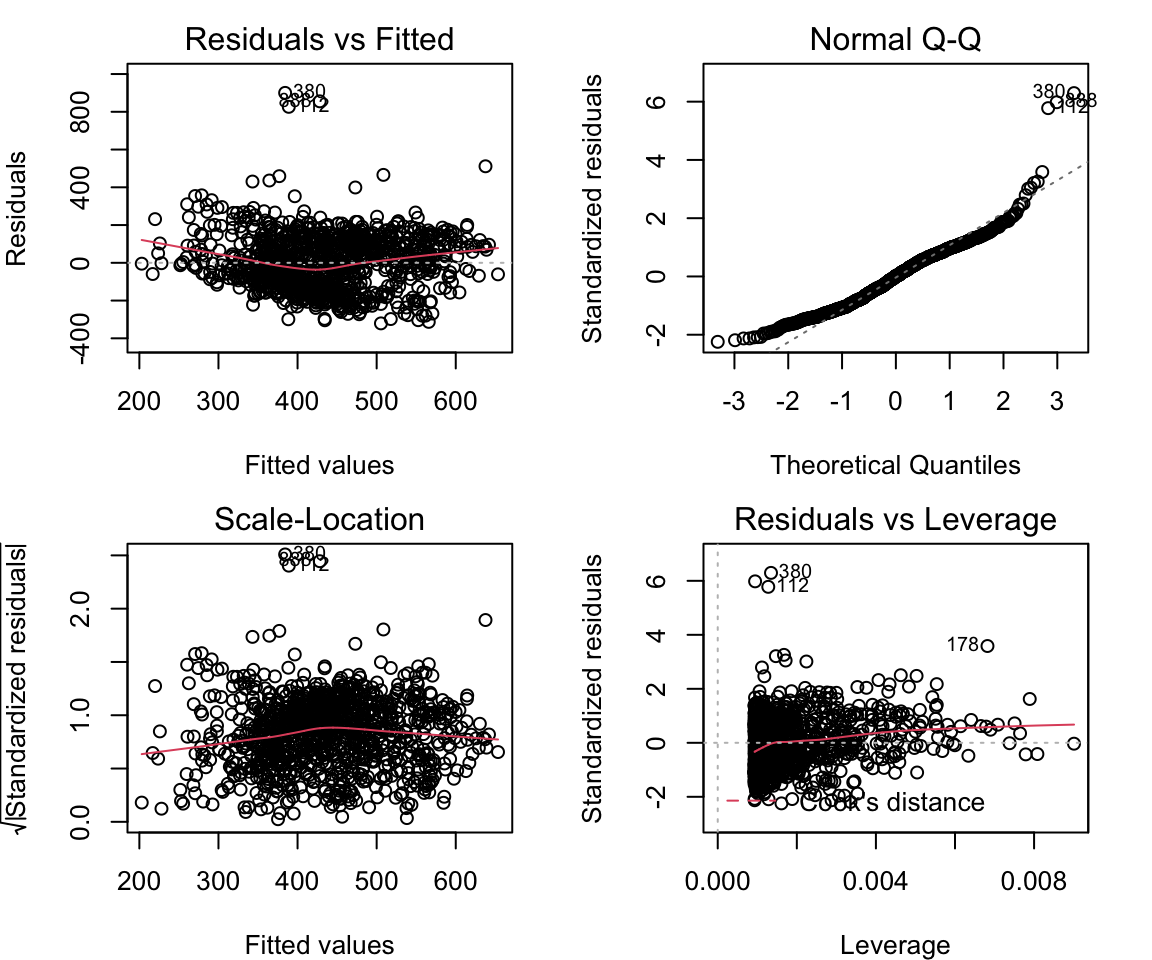
lmtest::bptest(lm1)##
## studentized Breusch-Pagan test
##
## data: lm1
## BP = 0.28531, df = 1, p-value = 0.5932Here, we see p > 0.05, so we cannot reject the null hypothesis, and therefore there is no significant heteroscedastity.
There are more assumptions, which I will not go into for the sake of time, but are discussed here:
https://www.r-bloggers.com/basic-assumptions-to-be-taken-care-of-when-building-a-predictive-model-2/
Moving beyond simple linear regression
What happens if we include more data in the model? For example, I only used the first tongue pellet here. What happens if we include all four tongue pellets in the analysis? Is this model better than the first one? We can compare models using anova() to see if they are different, and compare the R2 values.
lm2 = lm(f1~t1y+t2y+t3y+t4y, data = ubdb)
summary(lm2)
##
## Call:
## lm(formula = f1 ~ t1y + t2y + t3y + t4y, data = ubdb)
##
## Residuals:
## Min 1Q Median 3Q Max
## -414.33 -74.78 0.83 70.44 991.84
##
## Coefficients:
## Estimate Std. Error t value Pr(>|t|)
## (Intercept) 7.409e+02 1.800e+01 41.169 < 2e-16 ***
## t1y -1.155e-02 1.693e-03 -6.824 1.48e-11 ***
## t2y 9.897e-06 3.697e-03 0.003 0.998
## t3y -2.668e-04 4.052e-03 -0.066 0.948
## t4y -1.611e-02 2.409e-03 -6.686 3.69e-11 ***
## ---
## Signif. codes: 0 '***' 0.001 '**' 0.01 '*' 0.05 '.' 0.1 ' ' 1
##
## Residual standard error: 125.8 on 1068 degrees of freedom
## Multiple R-squared: 0.4116, Adjusted R-squared: 0.4094
## F-statistic: 186.8 on 4 and 1068 DF, p-value: < 2.2e-16bptest(lm2)##
## studentized Breusch-Pagan test
##
## data: lm2
## BP = 7.9782, df = 4, p-value = 0.09238anova(lm1, lm2)## Analysis of Variance Table
##
## Model 1: f1 ~ t1y
## Model 2: f1 ~ t1y + t2y + t3y + t4y
## Res.Df RSS Df Sum of Sq F Pr(>F)
## 1 1071 21937433
## 2 1068 16911652 3 5025781 105.8 < 2.2e-16 ***
## ---
## Signif. codes: 0 '***' 0.001 '**' 0.01 '*' 0.05 '.' 0.1 ' ' 1Here, what do the results mean? For each predictor, if we hold all other predictors constant and only increase the predictor in question by 1 unit, then f1 will change by the estimate of that predictor.
So, what would happen to f1 if we changed t2y by one unit? Is this a significant change in f1?
Interactions
Let’s try interactions. Interactions allow us assess the extent to which the association between one predictor and the outcome depends on a second predictor. For example, does the effect of tongue (tip) height on F1 also depend on tongue (dorsum) height?
lm3 = lm(f1~t1y*t4y, data = ubdb)
summary(lm3)
##
## Call:
## lm(formula = f1 ~ t1y * t4y, data = ubdb)
##
## Residuals:
## Min 1Q Median 3Q Max
## -423.89 -71.62 -6.74 72.11 967.31
##
## Coefficients:
## Estimate Std. Error t value Pr(>|t|)
## (Intercept) 7.230e+02 1.767e+01 40.923 < 2e-16 ***
## t1y -3.044e-02 3.301e-03 -9.222 < 2e-16 ***
## t4y -1.571e-02 9.092e-04 -17.282 < 2e-16 ***
## t1y:t4y 1.080e-06 1.846e-07 5.852 6.43e-09 ***
## ---
## Signif. codes: 0 '***' 0.001 '**' 0.01 '*' 0.05 '.' 0.1 ' ' 1
##
## Residual standard error: 123.8 on 1069 degrees of freedom
## Multiple R-squared: 0.4298, Adjusted R-squared: 0.4282
## F-statistic: 268.6 on 3 and 1069 DF, p-value: < 2.2e-16Categorical Predictors
What about categorical predictors? First, we need to make sure the categorical predictor is treated as a factor, not as a numeric. You can check that using the str() function. If you need to change the structure to factor, use the factor() function. This model includes the intercept as the vowel “AA.” Each estimate is the predicted change in f1 when going from AA to that vowel.
ubdb$v = factor(ubdb$v)
lm4 = lm(f1~v, data = ubdb)
summary(lm4)
##
## Call:
## lm(formula = f1 ~ v, data = ubdb)
##
## Residuals:
## Min 1Q Median 3Q Max
## -399.48 -68.30 2.01 78.64 900.18
##
## Coefficients:
## Estimate Std. Error t value Pr(>|t|)
## (Intercept) 618.86 14.92 41.491 < 2e-16 ***
## vAE -68.35 18.90 -3.617 0.000311 ***
## vAH -143.22 18.58 -7.709 2.90e-14 ***
## vAO -70.64 19.38 -3.645 0.000280 ***
## vEH -141.49 19.61 -7.216 1.02e-12 ***
## vIH -234.54 17.42 -13.463 < 2e-16 ***
## vIY -288.87 17.53 -16.482 < 2e-16 ***
## vUW -257.56 38.81 -6.637 5.09e-11 ***
## vUX -326.11 19.34 -16.859 < 2e-16 ***
## ---
## Signif. codes: 0 '***' 0.001 '**' 0.01 '*' 0.05 '.' 0.1 ' ' 1
##
## Residual standard error: 129.2 on 1064 degrees of freedom
## Multiple R-squared: 0.3823, Adjusted R-squared: 0.3777
## F-statistic: 82.32 on 8 and 1064 DF, p-value: < 2.2e-16Now we can integrate previous models together.
lm5 = lm(f1~t1y*t4y + v, data = ubdb)
summary(lm5)
##
## Call:
## lm(formula = f1 ~ t1y * t4y + v, data = ubdb)
##
## Residuals:
## Min 1Q Median 3Q Max
## -449.24 -62.87 -0.87 61.56 929.03
##
## Coefficients:
## Estimate Std. Error t value Pr(>|t|)
## (Intercept) 6.806e+02 2.257e+01 30.150 < 2e-16 ***
## t1y -2.860e-02 3.209e-03 -8.912 < 2e-16 ***
## t4y -7.953e-03 1.303e-03 -6.103 1.46e-09 ***
## vAE -3.899e+01 1.731e+01 -2.252 0.0245 *
## vAH -1.148e+02 1.699e+01 -6.754 2.36e-11 ***
## vAO -2.055e+01 1.825e+01 -1.126 0.2606
## vEH -8.432e+01 1.796e+01 -4.695 3.01e-06 ***
## vIH -1.193e+02 1.807e+01 -6.605 6.27e-11 ***
## vIY -1.541e+02 2.066e+01 -7.460 1.79e-13 ***
## vUW -1.761e+02 3.517e+01 -5.007 6.48e-07 ***
## vUX -1.953e+02 2.175e+01 -8.979 < 2e-16 ***
## t1y:t4y 1.067e-06 1.811e-07 5.892 5.13e-09 ***
## ---
## Signif. codes: 0 '***' 0.001 '**' 0.01 '*' 0.05 '.' 0.1 ' ' 1
##
## Residual standard error: 115.6 on 1061 degrees of freedom
## Multiple R-squared: 0.5065, Adjusted R-squared: 0.5014
## F-statistic: 98.99 on 11 and 1061 DF, p-value: < 2.2e-16anova(lm5, lm4)## Analysis of Variance Table
##
## Model 1: f1 ~ t1y * t4y + v
## Model 2: f1 ~ v
## Res.Df RSS Df Sum of Sq F Pr(>F)
## 1 1061 14184389
## 2 1064 17753182 -3 -3568794 88.983 < 2.2e-16 ***
## ---
## Signif. codes: 0 '***' 0.001 '**' 0.01 '*' 0.05 '.' 0.1 ' ' 1Predicting Values
One thing we can do with regression models is try to predict what the dependent variable would be, given certain values of the independent variable. To do this, we generate a data frame with the independent variables as columns, and their hypothetical values in each row. We then can use the predict() function to determine the predicted value, given the regression model. Note that you need a column for each predictor that exists in your model.
predictdata1 = with(ubdb,expand.grid(t1y = c(4444, 11111)))
head(predictdata1)
## t1y
## 1 4444
## 2 11111cbind(predictdata1, predict(lm1, type = "response",
se.fit = TRUE, interval="confidence",
newdata = predictdata1))## t1y fit.fit fit.lwr fit.upr se.fit df residual.scale
## 1 4444 364.8232 353.2212 376.4253 5.91284 1071 143.1193
## 2 11111 261.0065 240.1670 281.8461 10.62060 1071 143.1193predictdata5 = with(ubdb,expand.grid(t1y = c(4444, -2222), t4y =c(13213, 16161),v = c("AA", "UW")))
head(predictdata5)## t1y t4y v
## 1 4444 13213 AA
## 2 -2222 13213 AA
## 3 4444 16161 AA
## 4 -2222 16161 AA
## 5 4444 13213 UW
## 6 -2222 13213 UWcbind(predictdata5, predict(lm5, type = "response",
se.fit = TRUE, interval="confidence",
newdata = predictdata5))## t1y t4y v fit.fit fit.lwr fit.upr se.fit df residual.scale
## 1 4444 13213 AA 511.0152 480.3579 541.6724 15.62390 1061 115.6239
## 2 -2222 13213 AA 607.6958 581.4017 633.9899 13.40031 1061 115.6239
## 3 4444 16161 AA 501.5453 471.7848 531.3057 15.16686 1061 115.6239
## 4 -2222 16161 AA 577.2623 549.9431 604.5815 13.92271 1061 115.6239
## 5 4444 13213 UW 334.9478 270.6786 399.2170 32.75362 1061 115.6239
## 6 -2222 13213 UW 431.6284 367.8961 495.3606 32.47994 1061 115.6239
## 7 4444 16161 UW 325.4779 262.2974 388.6584 32.19876 1061 115.6239
## 8 -2222 16161 UW 401.1949 338.0526 464.3372 32.17929 1061 115.6239Binary Outcomes
Many linguistics experiments will have a binary outcome. In this case, our simple linear regression won’t work, as the lm() function takes only a continuous variable as its dependent variable. Therefore, we need to use another function - glm().
Let’s see if the f1 value can predict whether a vowel is a high or low vowel. First, we need to conditionally include this information. Then, we can run the model. We need to specify that this is a binomial model. (Note that if you want to run a model with three or more levels of your predictor variable, a binary logistic regression is no longer appropriate, and the model will not work. You need to use another type of analysis, such as a multinomial logistic regression, which I will not go into detail about here.)
mylevels = levels(ubdb$v)[1:4]
ubdb$vlow <- factor(ifelse(ubdb$v %in% mylevels,"LOW", "HIGH"))

glm1 = glm(vlow~f1+t1y, data = ubdb, family = "binomial")

glm2 = glm(vlow~f1+t1y+v, data = ubdb, family = "binomial")
## Warning: glm.fit: algorithm did not converge#what's wrong with this glm?
predictdata6 = with(ubdb,expand.grid(t1y = c(4444, -2222), f1 =c(666, 333)))
cbind(predictdata6, predict(glm1, type = "response",
se.fit = TRUE, interval="confidence",
newdata = predictdata6))## t1y f1 fit se.fit residual.scale
## 1 4444 666 0.6454607 0.04245873 1
## 2 -2222 666 0.7951722 0.02294796 1
## 3 4444 333 0.1570787 0.01576620 1
## 4 -2222 333 0.2843710 0.02275635 1Polynomial Regression
Sometimes, a linear line might not be considered the best model of our data. There are multiple ways of modeling data besides a linear relationship, including higher-order polynomials. We can include the polynomial in the lm() function, because even though we are fitting a higher-order line to the data, the model still falls in the linear regression family because the relationship between coefficients is linear. (Examples of nonlinear regressions inclue exponential, and logarithmic regressions.)
lm7 = lm(f1~t1y + I(t1y^2), data = ubdb)
summary(lm7)
##
## Call:
## lm(formula = f1 ~ t1y + I(t1y^2), data = ubdb)
##
## Residuals:
## Min 1Q Median 3Q Max
## -343.20 -108.72 -4.84 105.93 910.47
##
## Coefficients:
## Estimate Std. Error t value Pr(>|t|)
## (Intercept) 4.127e+02 5.350e+00 77.139 < 2e-16 ***
## t1y -1.473e-02 8.471e-04 -17.390 < 2e-16 ***
## I(t1y^2) 8.205e-07 1.232e-07 6.658 4.42e-11 ***
## ---
## Signif. codes: 0 '***' 0.001 '**' 0.01 '*' 0.05 '.' 0.1 ' ' 1
##
## Residual standard error: 140.3 on 1070 degrees of freedom
## Multiple R-squared: 0.2671, Adjusted R-squared: 0.2657
## F-statistic: 195 on 2 and 1070 DF, p-value: < 2.2e-16f <- function(x,c) coef(lm7)[1] + coef(lm7)[2]*x + coef(lm7)[3]*x^2
pl <- ggplot(ubdb) + geom_point(aes(x=t1y, y=f1), size=2, colour="#993399") + geom_abline(intercept=coef(lm1)[1],slope=coef(lm1)[2],size=1, colour="#339900") +
stat_function(fun=f, colour="red", size=1)+ylim(c(0,2000))Mixed Effects Models
The type of model that is used most often in linguistics research is the mixed effects model. Mixed effects models have two types of independent variables: fixed effects and random effects. For fixed effects, the observed values are of direct interest. For example, vowel quality, experimental condition, language background, etc., can be considered a fixed effect. In this example, v is a fixed effect. Random effects, on the other hand, are not of direct interest in the model. The goal is to make inferences to a general population based on the observed differences between levels. Speaker or participant is a common random effect.
How do we encode random effects? It depends on what you are trying to do. First, running a null model (with only random effects, but no fixed effects), allows a preliminary understanding of the variance between levels of the random effect. Because the current dataset does not have any random effects, I have “created” them.
myspeakers = c("S1", "S2", "S3", "S4", "S5")
ubdb$speaker = factor(sample(myspeakers, dim(ubdb)[1], replace = TRUE))
lme1= lmer(f1~1+(1|speaker), data = ubdb, REML = FALSE)
## boundary (singular) fit: see ?isSingularsummary(lme1) ## Linear mixed model fit by maximum likelihood . t-tests use Satterthwaite's
## method [lmerModLmerTest]
## Formula: f1 ~ 1 + (1 | speaker)
## Data: ubdb
##
## AIC BIC logLik deviance df.resid
## 13991.0 14005.9 -6992.5 13985.0 1070
##
## Scaled residuals:
## Min 1Q Median 3Q Max
## -2.1271 -0.8934 -0.0448 0.7746 5.1757
##
## Random effects:
## Groups Name Variance Std.Dev.
## speaker (Intercept) 0 0.0
## Residual 26786 163.7
## Number of obs: 1073, groups: speaker, 5
##
## Fixed effects:
## Estimate Std. Error df t value Pr(>|t|)
## (Intercept) 437.433 4.996 1073.000 87.55 <2e-16 ***
## ---
## Signif. codes: 0 '***' 0.001 '**' 0.01 '*' 0.05 '.' 0.1 ' ' 1
## convergence code: 0
## boundary (singular) fit: see ?isSingularThe variance in random factor tells you how much variability there is between individuals across all vowels, not the level of variance between individuals within each vowel category.
Now let’s see if we can model f1 based on tongue position and speaker.
lme2= lmer(f1~t1y+(1|speaker), data = ubdb, REML = FALSE)## Warning: Some predictor variables are on very different scales: consider
## rescaling## boundary (singular) fit: see ?isSingular## Warning: Some predictor variables are on very different scales: consider
## rescalingsummary(lme2) ## Linear mixed model fit by maximum likelihood . t-tests use Satterthwaite's
## method [lmerModLmerTest]
## Formula: f1 ~ t1y + (1 | speaker)
## Data: ubdb
##
## AIC BIC logLik deviance df.resid
## 13703.1 13723.0 -6847.5 13695.1 1069
##
## Scaled residuals:
## Min 1Q Median 3Q Max
## -2.2438 -0.7848 0.0085 0.7143 6.2958
##
## Random effects:
## Groups Name Variance Std.Dev.
## speaker (Intercept) 0 0
## Residual 20445 143
## Number of obs: 1073, groups: speaker, 5
##
## Fixed effects:
## Estimate Std. Error df t value Pr(>|t|)
## (Intercept) 4.340e+02 4.369e+00 1.073e+03 99.34 <2e-16 ***
## t1y -1.557e-02 8.536e-04 1.073e+03 -18.24 <2e-16 ***
## ---
## Signif. codes: 0 '***' 0.001 '**' 0.01 '*' 0.05 '.' 0.1 ' ' 1
##
## Correlation of Fixed Effects:
## (Intr)
## t1y 0.043
## fit warnings:
## Some predictor variables are on very different scales: consider rescaling
## convergence code: 0
## boundary (singular) fit: see ?isSingularubdb$t1y.z = scale(ubdb$t1y,center = TRUE, scale = TRUE)
lme3= lmer(f1~t1y.z+(1|speaker), data = ubdb, REML = FALSE)## boundary (singular) fit: see ?isSingularsummary(lme3) ## Linear mixed model fit by maximum likelihood . t-tests use Satterthwaite's
## method [lmerModLmerTest]
## Formula: f1 ~ t1y.z + (1 | speaker)
## Data: ubdb
##
## AIC BIC logLik deviance df.resid
## 13703.1 13723.0 -6847.5 13695.1 1069
##
## Scaled residuals:
## Min 1Q Median 3Q Max
## -2.2438 -0.7848 0.0085 0.7143 6.2958
##
## Random effects:
## Groups Name Variance Std.Dev.
## speaker (Intercept) 0 0
## Residual 20445 143
## Number of obs: 1073, groups: speaker, 5
##
## Fixed effects:
## Estimate Std. Error df t value Pr(>|t|)
## (Intercept) 437.433 4.365 1073.000 100.21 <2e-16 ***
## t1y.z -79.667 4.367 1073.000 -18.24 <2e-16 ***
## ---
## Signif. codes: 0 '***' 0.001 '**' 0.01 '*' 0.05 '.' 0.1 ' ' 1
##
## Correlation of Fixed Effects:
## (Intr)
## t1y.z 0.000
## convergence code: 0
## boundary (singular) fit: see ?isSingularlme5= lmer(f1~t1y.z+v+(1|speaker), data = ubdb, REML = FALSE)## boundary (singular) fit: see ?isSingularsummary(lme5) ## Linear mixed model fit by maximum likelihood . t-tests use Satterthwaite's
## method [lmerModLmerTest]
## Formula: f1 ~ t1y.z + v + (1 | speaker)
## Data: ubdb
##
## AIC BIC logLik deviance df.resid
## 13335.5 13395.2 -6655.8 13311.5 1061
##
## Scaled residuals:
## Min 1Q Median 3Q Max
## -3.2685 -0.6003 0.0203 0.5899 7.6046
##
## Random effects:
## Groups Name Variance Std.Dev.
## speaker (Intercept) 0 0.0
## Residual 14300 119.6
## Number of obs: 1073, groups: speaker, 5
##
## Fixed effects:
## Estimate Std. Error df t value Pr(>|t|)
## (Intercept) 591.608 13.967 1073.000 42.358 < 2e-16 ***
## t1y.z -53.010 4.084 1073.000 -12.981 < 2e-16 ***
## vAE -61.230 17.501 1073.000 -3.499 0.000487 ***
## vAH -146.953 17.202 1073.000 -8.543 < 2e-16 ***
## vAO -70.465 17.940 1073.000 -3.928 9.12e-05 ***
## vEH -113.316 18.281 1073.000 -6.198 8.12e-10 ***
## vIH -181.115 16.644 1073.000 -10.882 < 2e-16 ***
## vIY -235.341 16.741 1073.000 -14.058 < 2e-16 ***
## vUW -216.232 36.066 1073.000 -5.995 2.77e-09 ***
## vUX -291.066 18.109 1073.000 -16.073 < 2e-16 ***
## ---
## Signif. codes: 0 '***' 0.001 '**' 0.01 '*' 0.05 '.' 0.1 ' ' 1
##
## Correlation of Fixed Effects:
## (Intr) t1y.z vAE vAH vAO vEH vIH vIY vUW
## t1y.z 0.150
## vAE -0.785 -0.031
## vAH -0.791 0.017 0.633
## vAO -0.761 -0.001 0.607 0.618
## vEH -0.765 -0.119 0.600 0.604 0.581
## vIH -0.857 -0.247 0.662 0.662 0.639 0.656
## vIY -0.852 -0.246 0.658 0.658 0.635 0.652 0.745
## vUW -0.392 -0.088 0.305 0.306 0.295 0.300 0.339 0.338
## vUX -0.776 -0.149 0.606 0.610 0.587 0.594 0.669 0.666 0.305
## convergence code: 0
## boundary (singular) fit: see ?isSingularIn this sets of models, each contains a random intercept shared by individuals that have the same value for speaker - each speaker’s regression line is shifted up/down by a random amount with mean 0. This implies that each speaker shows the same relationship (i.e., slope) between t1y and f1, but at a different “starting” point.
What if we want to include a random slope, meaning that speaker’s F1 differs at different rates based on t1y. Then we would run the following code:
lme6= lmer(f1~t1y.z+v+(1+t1y.z|speaker), data = ubdb, REML = FALSE)## boundary (singular) fit: see ?isSingularsummary(lme6) ## Linear mixed model fit by maximum likelihood . t-tests use Satterthwaite's
## method [lmerModLmerTest]
## Formula: f1 ~ t1y.z + v + (1 + t1y.z | speaker)
## Data: ubdb
##
## AIC BIC logLik deviance df.resid
## 13339.4 13409.1 -6655.7 13311.4 1059
##
## Scaled residuals:
## Min 1Q Median 3Q Max
## -3.2606 -0.5938 0.0191 0.5872 7.6138
##
## Random effects:
## Groups Name Variance Std.Dev. Corr
## speaker (Intercept) 1.901 1.379
## t1y.z 10.351 3.217 1.00
## Residual 14287.549 119.531
## Number of obs: 1073, groups: speaker, 5
##
## Fixed effects:
## Estimate Std. Error df t value Pr(>|t|)
## (Intercept) 591.404 13.979 1002.608 42.305 < 2e-16 ***
## t1y.z -52.961 4.329 9.388 -12.234 4.43e-07 ***
## vAE -61.218 17.498 1070.462 -3.499 0.000487 ***
## vAH -146.782 17.201 1072.187 -8.534 < 2e-16 ***
## vAO -70.381 17.936 1070.565 -3.924 9.26e-05 ***
## vEH -112.993 18.281 1072.392 -6.181 9.05e-10 ***
## vIH -180.996 16.642 1071.561 -10.876 < 2e-16 ***
## vIY -235.174 16.736 1069.591 -14.052 < 2e-16 ***
## vUW -216.253 36.058 1071.323 -5.997 2.74e-09 ***
## vUX -290.908 18.106 1071.196 -16.067 < 2e-16 ***
## ---
## Signif. codes: 0 '***' 0.001 '**' 0.01 '*' 0.05 '.' 0.1 ' ' 1
##
## Correlation of Fixed Effects:
## (Intr) t1y.z vAE vAH vAO vEH vIH vIY vUW
## t1y.z 0.156
## vAE -0.784 -0.029
## vAH -0.790 0.016 0.633
## vAO -0.760 -0.001 0.607 0.618
## vEH -0.764 -0.111 0.600 0.605 0.582
## vIH -0.857 -0.233 0.662 0.662 0.639 0.656
## vIY -0.852 -0.232 0.658 0.658 0.635 0.652 0.745
## vUW -0.391 -0.083 0.305 0.306 0.295 0.300 0.339 0.338
## vUX -0.776 -0.140 0.606 0.610 0.587 0.594 0.670 0.666 0.305
## convergence code: 0
## boundary (singular) fit: see ?isSingularThis model, in addition to a random intercept, also contains a random slope for t1y. This means that the rate of f1 change based on t1y is different from person to person. If an individual has a positive random effect, then their f1 increases more quickly with practice than the average, while a negative random effect indicates their f1 increases less quickly with practice than the average.
To constrain the model so that the random slope and random intercept are uncorrelated (and therefore independent, since they are normally distributed), you’d fit the model:
lme6= lmer(f1~t1y.z+v+(1|speaker)+(t1y.z-1|speaker), data = ubdb, REML = FALSE)## boundary (singular) fit: see ?isSingularsummary(lme6) ## Linear mixed model fit by maximum likelihood . t-tests use Satterthwaite's
## method [lmerModLmerTest]
## Formula: f1 ~ t1y.z + v + (1 | speaker) + (t1y.z - 1 | speaker)
## Data: ubdb
##
## AIC BIC logLik deviance df.resid
## 13337.5 13402.2 -6655.8 13311.5 1060
##
## Scaled residuals:
## Min 1Q Median 3Q Max
## -3.2658 -0.6002 0.0217 0.5882 7.6057
##
## Random effects:
## Groups Name Variance Std.Dev.
## speaker (Intercept) 0.000 0.000
## speaker.1 t1y.z 2.173 1.474
## Residual 14297.609 119.573
## Number of obs: 1073, groups: speaker, 5
##
## Fixed effects:
## Estimate Std. Error df t value Pr(>|t|)
## (Intercept) 591.567 13.968 1069.867 42.353 < 2e-16 ***
## t1y.z -52.995 4.137 8.600 -12.811 6.74e-07 ***
## vAE -61.248 17.502 1071.977 -3.500 0.000485 ***
## vAH -146.926 17.202 1071.616 -8.541 < 2e-16 ***
## vAO -70.432 17.940 1072.977 -3.926 9.19e-05 ***
## vEH -113.263 18.282 1071.966 -6.195 8.28e-10 ***
## vIH -181.092 16.644 1071.943 -10.880 < 2e-16 ***
## vIY -235.301 16.741 1072.954 -14.056 < 2e-16 ***
## vUW -216.227 36.065 1071.030 -5.996 2.77e-09 ***
## vUX -291.033 18.110 1072.832 -16.071 < 2e-16 ***
## ---
## Signif. codes: 0 '***' 0.001 '**' 0.01 '*' 0.05 '.' 0.1 ' ' 1
##
## Correlation of Fixed Effects:
## (Intr) t1y.z vAE vAH vAO vEH vIH vIY vUW
## t1y.z 0.148
## vAE -0.785 -0.031
## vAH -0.791 0.017 0.633
## vAO -0.761 -0.001 0.607 0.618
## vEH -0.765 -0.117 0.600 0.604 0.581
## vIH -0.857 -0.244 0.662 0.662 0.639 0.656
## vIY -0.852 -0.243 0.658 0.658 0.635 0.652 0.745
## vUW -0.392 -0.087 0.305 0.306 0.295 0.300 0.339 0.338
## vUX -0.776 -0.147 0.606 0.610 0.587 0.594 0.669 0.666 0.305
## convergence code: 0
## boundary (singular) fit: see ?isSingular