R Graphing Workshop
The aim of this workshop is to teach you the ins and outs of using the ggplot2 package in R.
The materials for this workshop can be found here.
A lot of the information in this workshop is based on workshops given at Harvard: https://dss.iq.harvard.edu/workshop-materials
Please make good use of the following cheat sheet! https://www.rstudio.com/wp-content/uploads/2015/03/ggplot2-cheatsheet.pdf
Data
The data I will be using during this tutorial is from the University of Wisconsin’s X-Ray Microbeam Speech Production Database. The database has the following variables:
- v = vowel
- f0
- f1-f4
- ulx and uly = x and y coordinates of the upper lip
- llx and lly = x and y coordinates of the lower lip
- t(1-4)x and t(1-4)y = x and y coordinates of the tongue at position (1-4)
- mnix and mniy = x and y coordinates of the mandibular incisor
- mnmx and mnmy = x and y coordinates of the mandibular molar
- I have artificially introduced 5 “speakers” randomly
Introduction to ggplot
As linguists, we are often dealing with data. And dealing with data means that when we are presenting results, we need to both describe these results in words, and display these results using plots.
R is very powerful when it comes to making graphics. There are a lot of functions in base R that can create these graphics:
hist(ubdb$f1)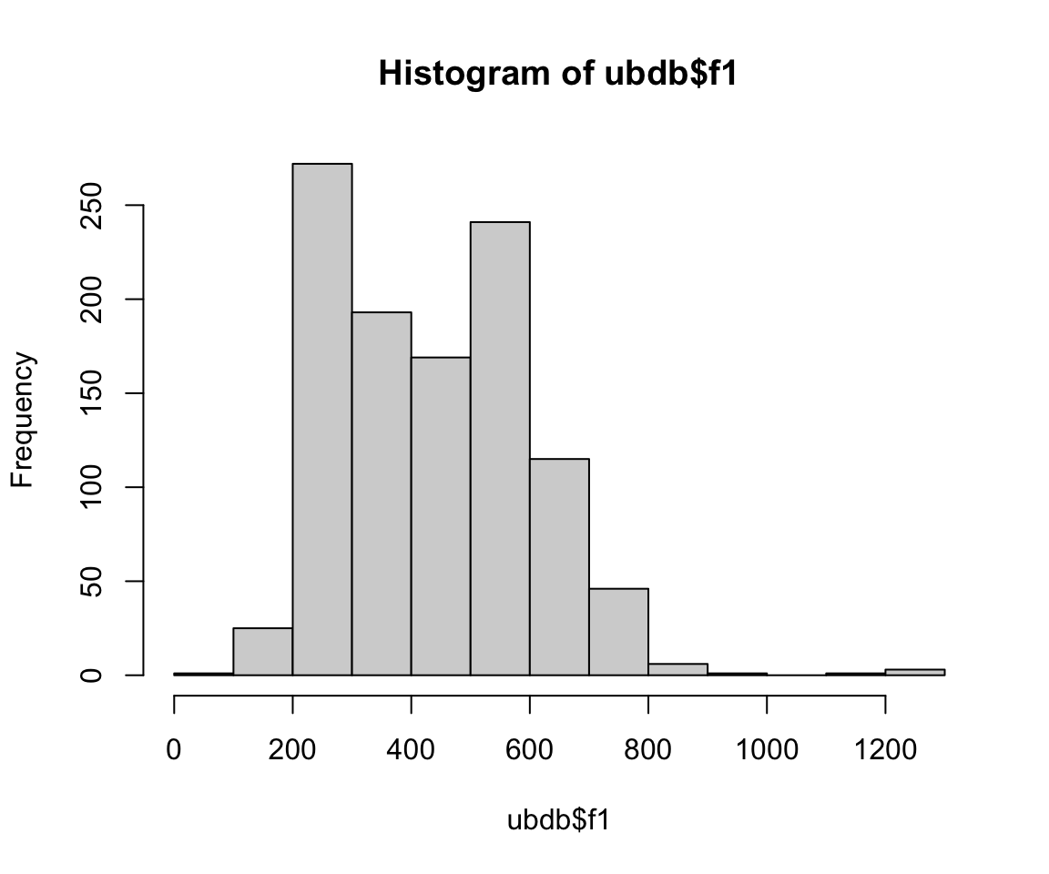
plot(ubdb$t1y, ubdb$f1)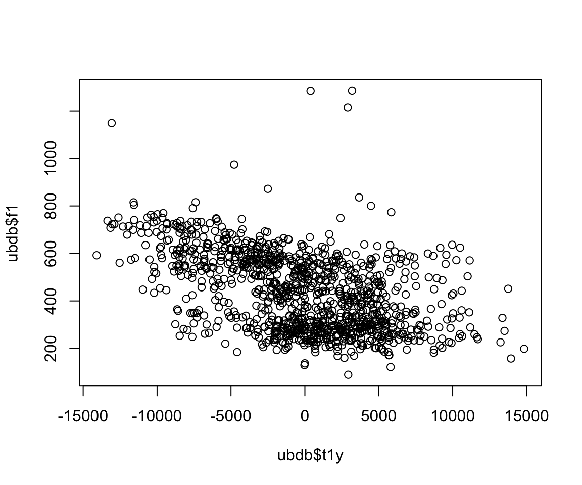
boxplot(f1~v, notch = TRUE, data = ubdb)## Warning in bxp(list(stats = structure(c(419.198, 574.662, 611.469, 698.7815, :
## some notches went outside hinges ('box'): maybe set notch=FALSE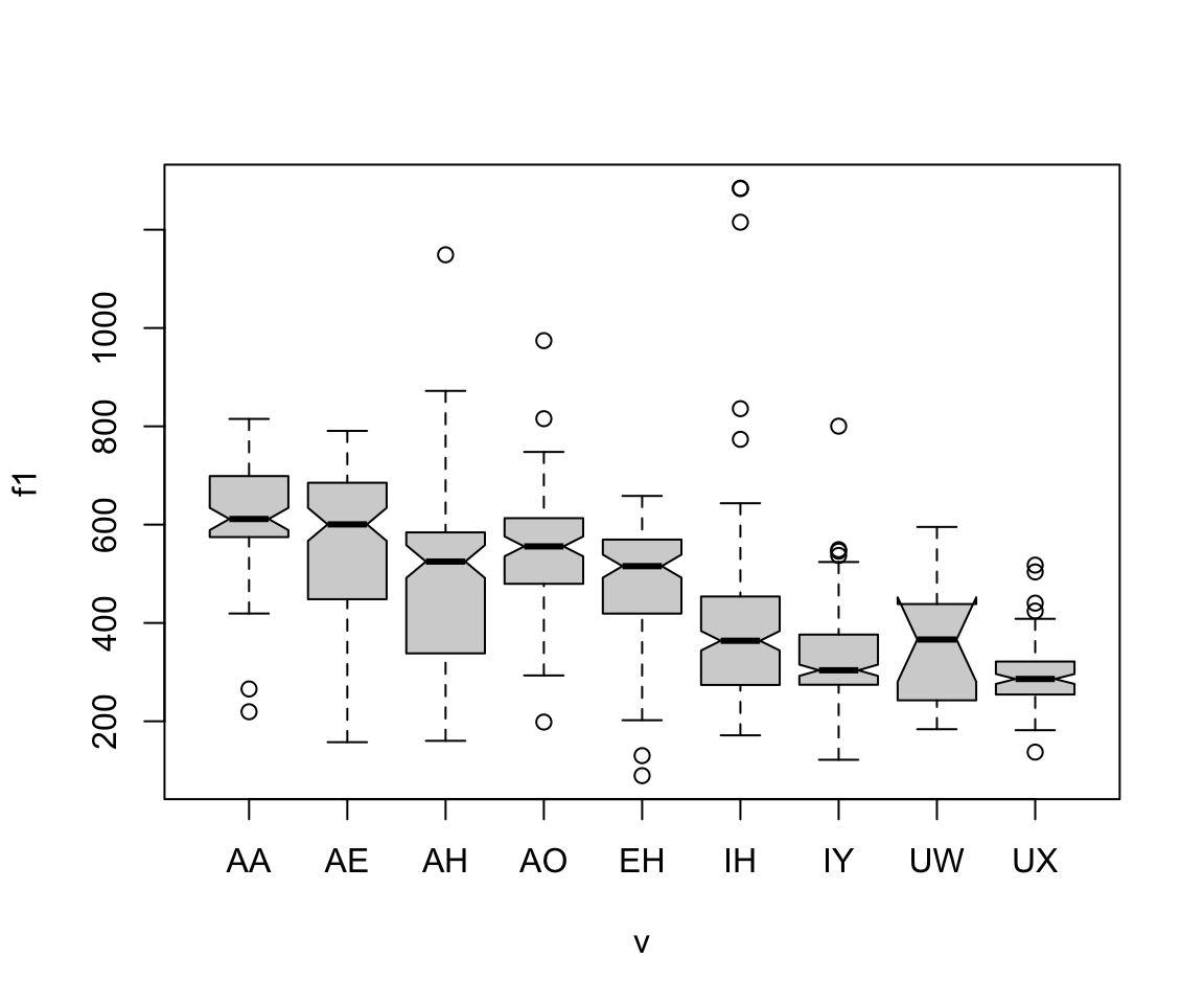
However, each of these functions have slightly different syntactic forms, and the code is more complex to create plots. The ggplot() function, on the other hand, has a consistent coding structure, and creates much prettier plots. Once you understand the basic functions in ggplot, pretty and informative graphics are only a few steps away!
The basic idea is similar to that of Photoshop. You independently specify building blocks of your plot, and combine them to create a graphical display. We add these building blocks (i.e., layers) to the graph using the “+” sign. Building blocks include:
- data
- aesthetic mapping
- geometric object
- statistical transformations
- scales
- coordinate systems
- position adjustments
- faceting
It is important to include everything you need in one data frame for the graph. The first thing that happens is you call the data frame, and every subsequent call for a variable will come directly from that data frame.
Aesthetics
In ggplot(), aesthetics include things you can see. Aesthetics are called with the function aes(). Some example aesthetics are:
- x: positioning along x-axis
- y: positioning along y-axis
- color: color of objects, or the color of the object’s outline (compare to fill below)
- fill: fill color of objects
- alpha: transparency of objects (value between 0, transparent, and 1, opaque)
- linetype: how lines should be drawn (solid, dashed, dotted, etc.)
- shape: shape of markers in scatter plots
- size: how large objects appear
Let’s see what happens when we use ggplot() and aes() together:
ggplot(ubdb, aes(x=t1y, y=f1))
What’s going on here? We’ve told ggplot to make a graph for the data file ubdb, with the x axis being t1y, and the y axis being f1. However, we didn’t specify what kind of graph we want. There are a few options for this, many of which are considered geometric objects:
- geom_point()
- geom_boxplot()
- geom_line()
- geom_ribbon()
- geom_label() or geom_text()
- geom_violin()
Let’s try some of these:
ggplot(ubdb, aes(x=t1y, y=f1)) + geom_point()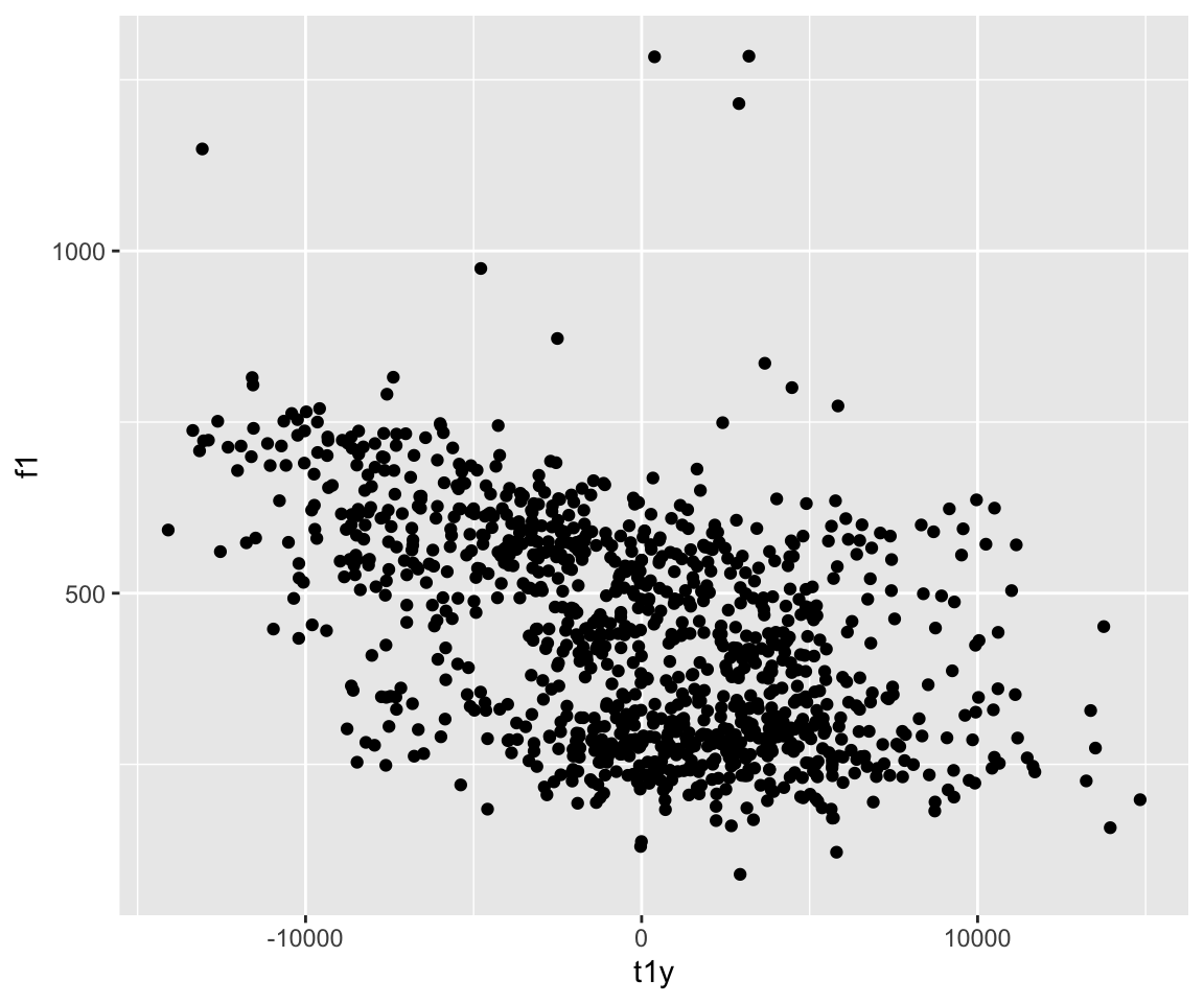
ggplot(ubdb, aes(x=t1y, y=f1)) + geom_point(aes(color = v))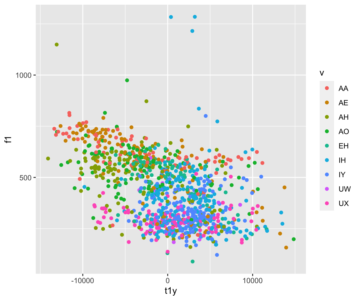
ggplot(ubdb, aes(x=t1y, y=f1)) + geom_point(aes(color = f1))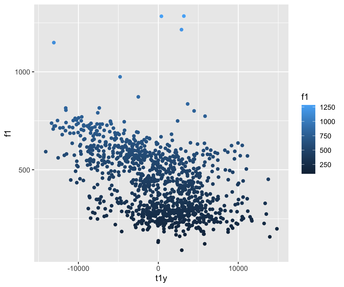
ggplot(ubdb, aes(x=t1y, y=f1)) + geom_point(aes(color = t4y))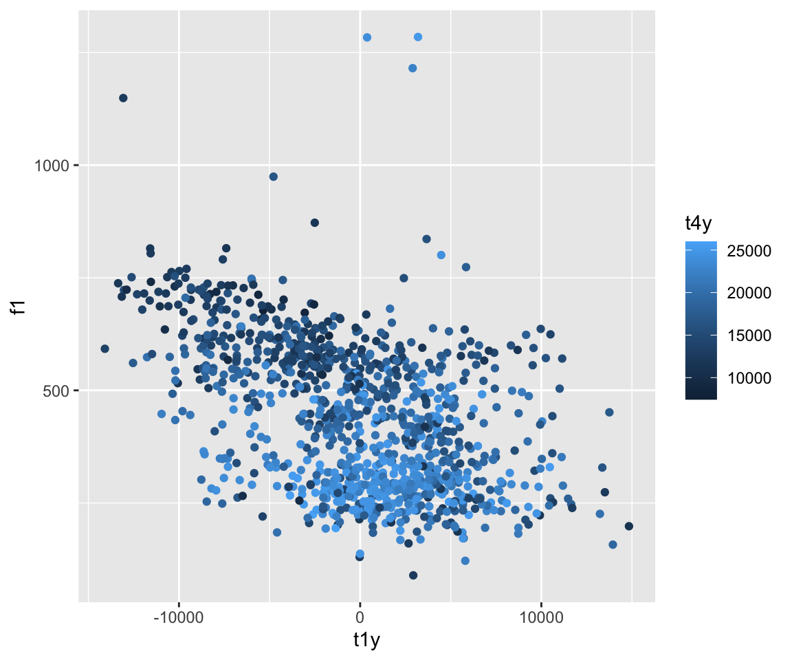 What’s the difference here? For the first plot, we are plotting basic geometric points. For the subsequent plots, we are adding an additional layer to the plot - changing the color of the plots from the default black. Therefore, the aesthetics of the points need to be included.
ggplot(ubdb, aes(x=t1y, y=f1)) + geom_point(aes(color = t4y, size = 2))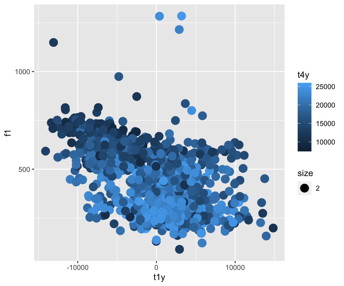
ggplot(ubdb, aes(x=t1y, y=f1)) + geom_point(aes(color = t4y), size = 2)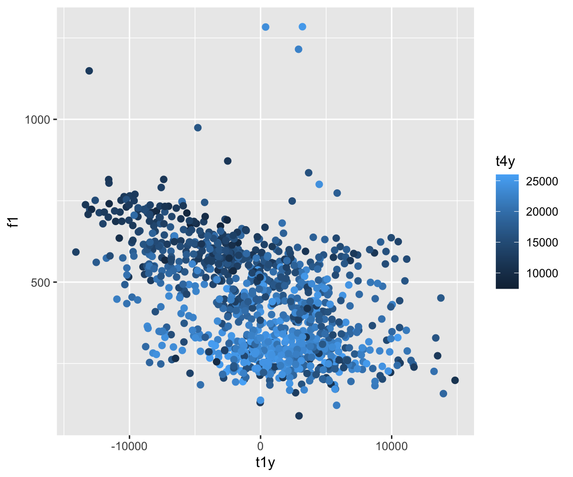
Here, the size is included as a variable, which is why we end up with an extra legend. Therefore, it is important to keep any aesthetics that do not call a variable (i.e., are fixed for the entire plot) stay outside of the aes() call. If you want to to base size on a variable (or color, linetype, etc.)) but do not want the legend, you can use guides() after your call for that geometric object, and specify which guide you do not want to be shown by using FLASE.
ggplot(ubdb, aes(x=t1y, y=f1)) + geom_point(aes(color = t4y, size = t1y))+guides(size = FALSE)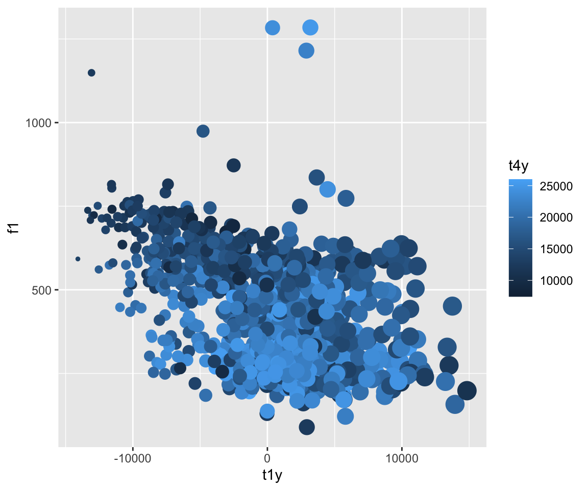
ggplot(ubdb, aes(x=t1y, y=f1)) + geom_point(aes(color = t4y, size = t1y))+guides(color = FALSE)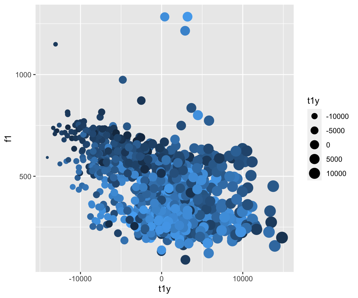
So what’s going on here? Why do we get an error for the second plot call?
ggplot(ubdb, aes(x=t1y, y=f1)) + geom_line(group = v, color = v)## Error in layer(data = data, mapping = mapping, stat = stat, geom = GeomLine, : object 'v' not found#This is one way to get around the aes() issue, but is not the best! It means you have to call your data file again, and if you have some similarly-titled data frames, a simple typo can give you an inaccurate graph!
ggplot(ubdb, aes(x=t1y, y=f1)) + geom_line(group = ubdb$v, color = ubdb$v)## Error: Unknown colour name: AA#This is the best method of doing it!
ggplot(ubdb, aes(x=t1y, y=f1)) + geom_line(aes(group = v, color = v))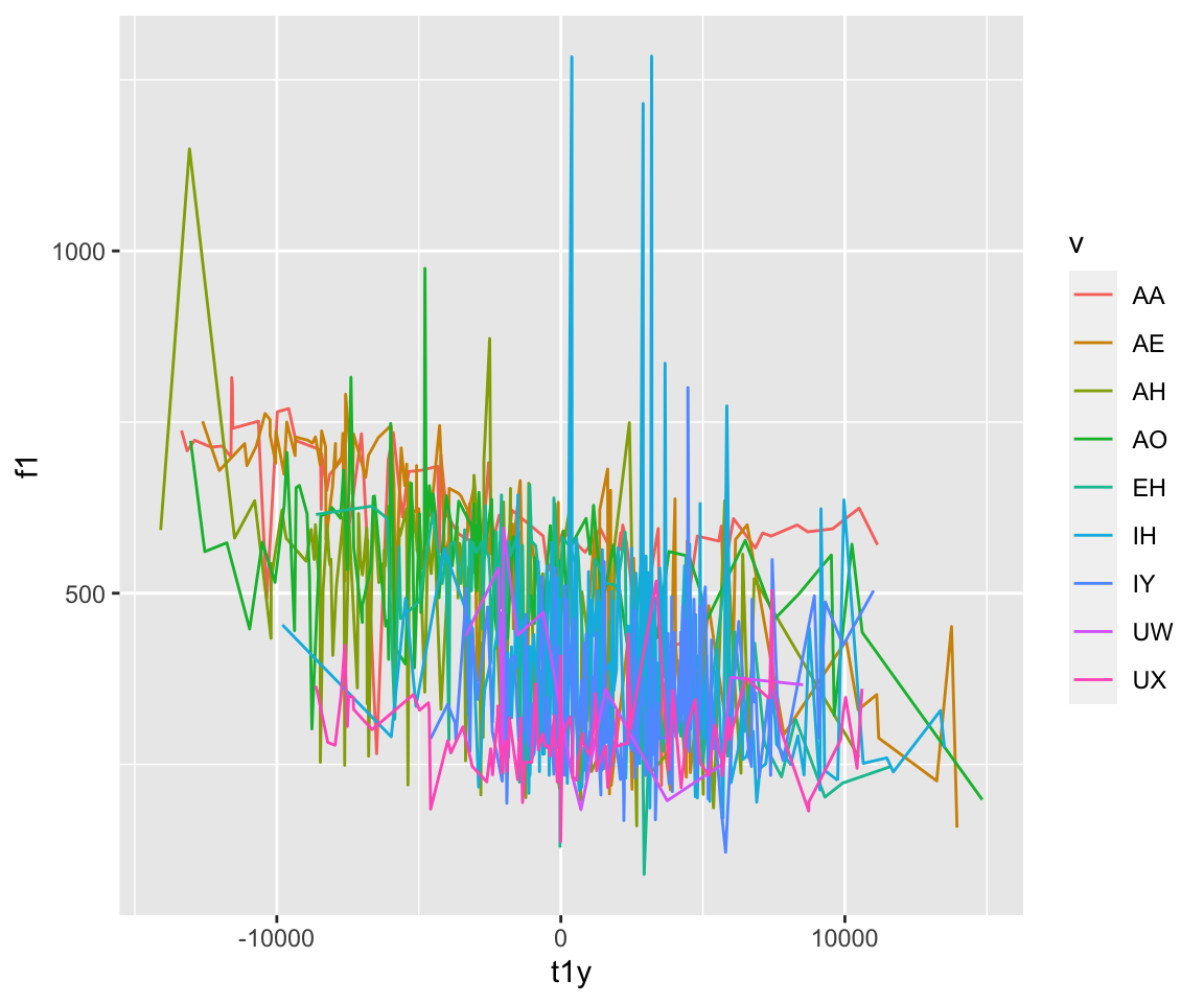
What about other aesthetics?
For boxplots and barplots, as well as other geoms, we can include significance levels with the ggsignif package. The pairwise comparisons being made are included in a list. The significance levels can be manually given using the ‘annotations’ argument. The geom_signif function has many other possibilities for changing the style of the significance bars.
ggplot(ubdb, aes(x=v, y=f1)) + geom_boxplot(aes(group = v))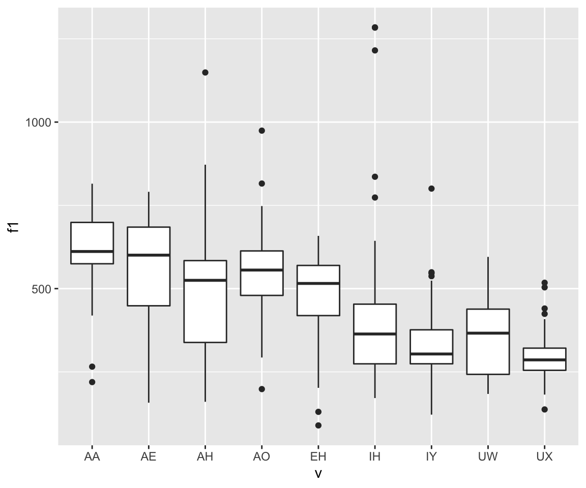
mycomparisons = list(c("AA", "AE"), c("IH", "IY"), c("IH", "UW"))
ggplot(ubdb, aes(x=v, y=f1)) + geom_boxplot(aes(group = v)) + geom_signif(comparisons = mycomparisons, annotations = c("***", "**", "NS"), y = c(1000, 1500, 1000))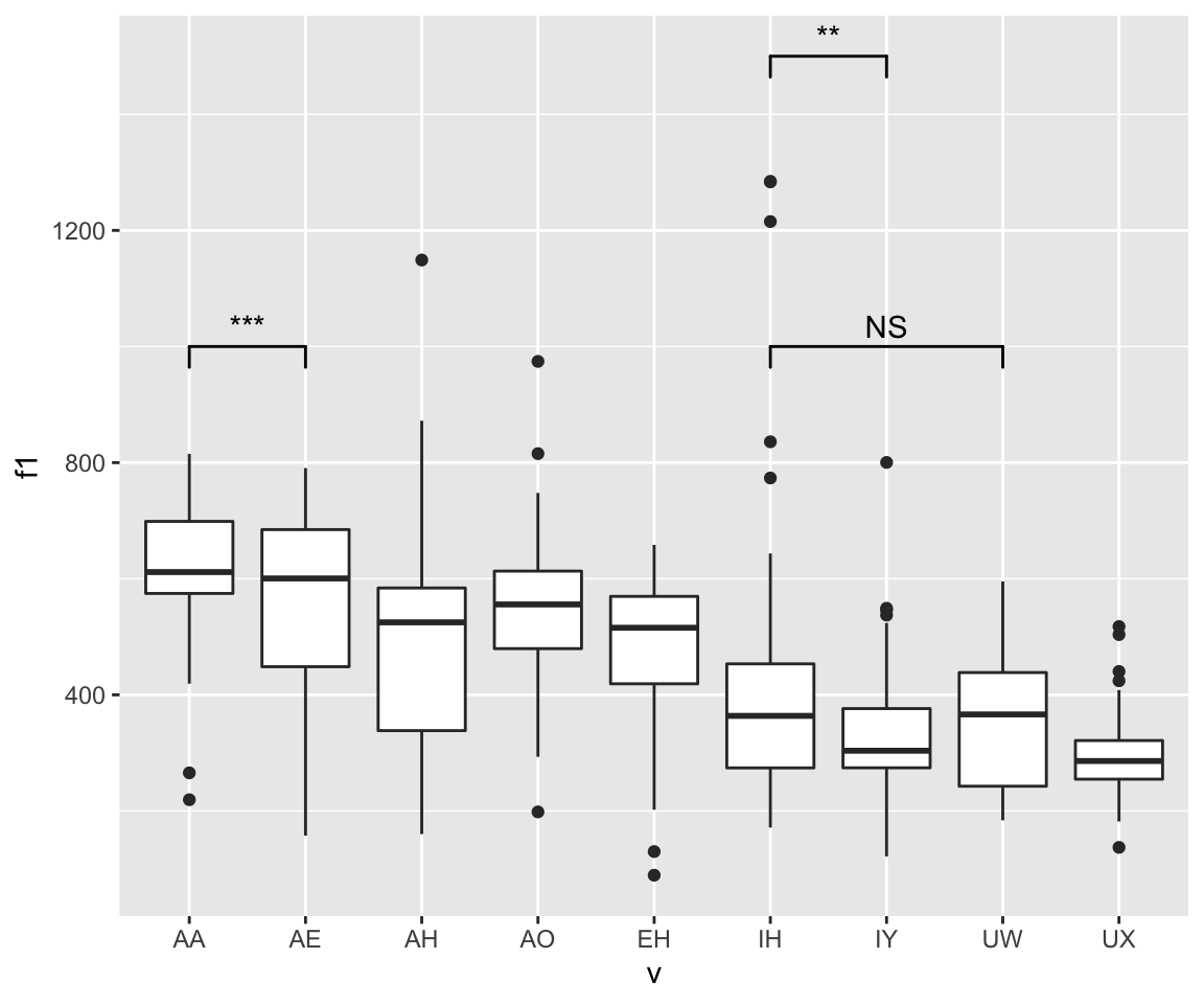
ggplot(ubdb, aes(x=t1y, fill=v)) + geom_density(size = 1, alpha=.2)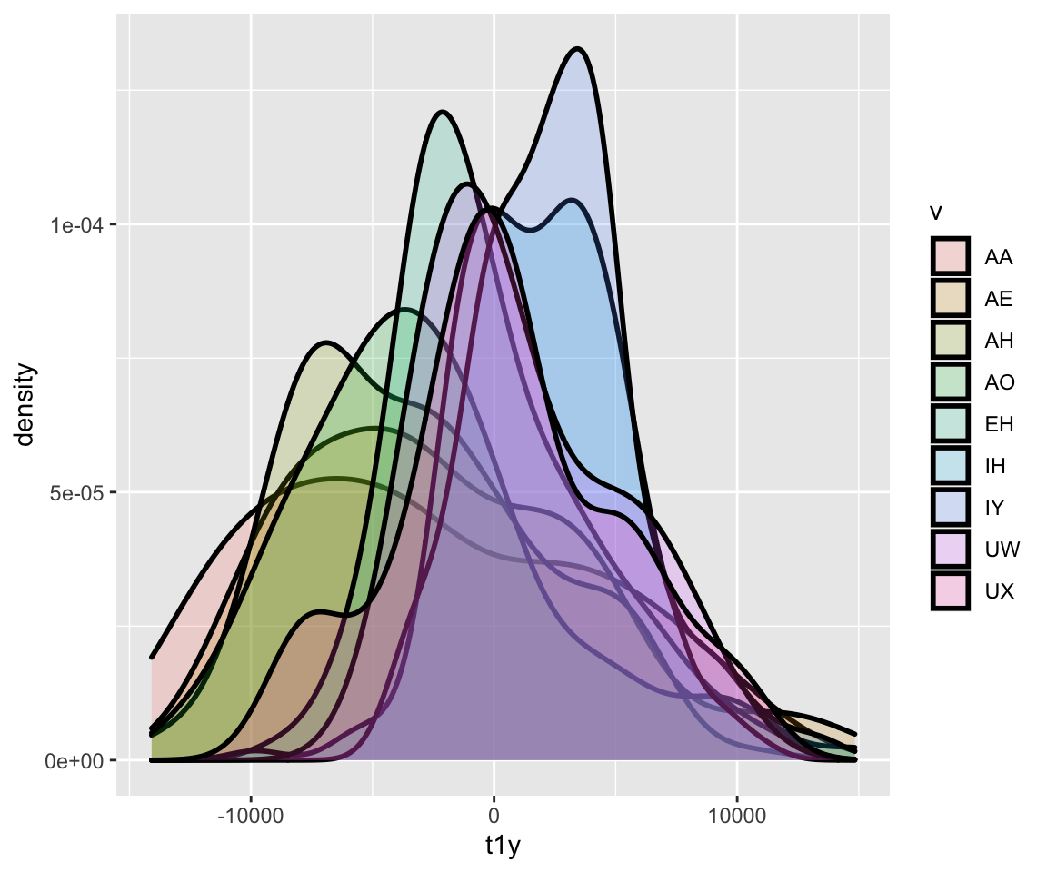
The following plots are going to look pretty darn ugly! Why is that? What can we do to fix them?
ggplot(ubdb, aes(x=t1y, y=f1)) + geom_line(aes(group = v))+geom_ribbon(aes(group = v, ymin = f1-sd(f1), ymax = f1+sd(f1)))
ggplot(ubdb, aes(x=t1y, y=f1)) + geom_line(aes(group = v))+geom_smooth(aes(group =v, color = v))## `geom_smooth()` using method = 'loess' and formula 'y ~ x'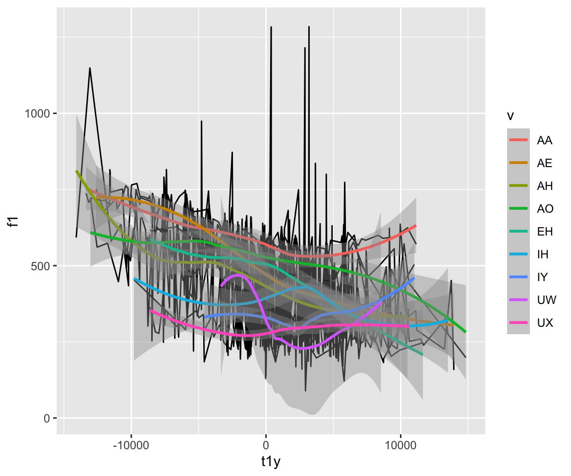
ggplot(ubdb, aes(x=t1y, y=f1)) + geom_smooth(aes(color = v), method = "gam", size = 2)+geom_ribbon(aes(color = v, ymin = f1-sd(f1), ymax = f1+sd(f1)), alpha = .2)## `geom_smooth()` using formula 'y ~ s(x, bs = "cs")'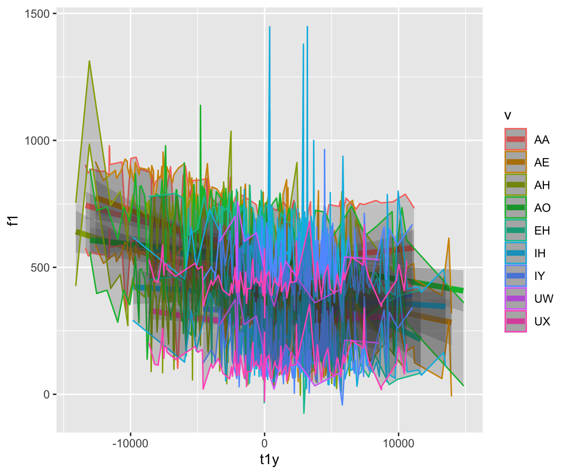
#this is better. There is not an overload of information in these plots!
ggplot(ubdb, aes(x=t1y, y=f1)) + geom_smooth(aes(color = v), method = "gam", size = 2)
## `geom_smooth()` using formula 'y ~ s(x, bs = "cs")'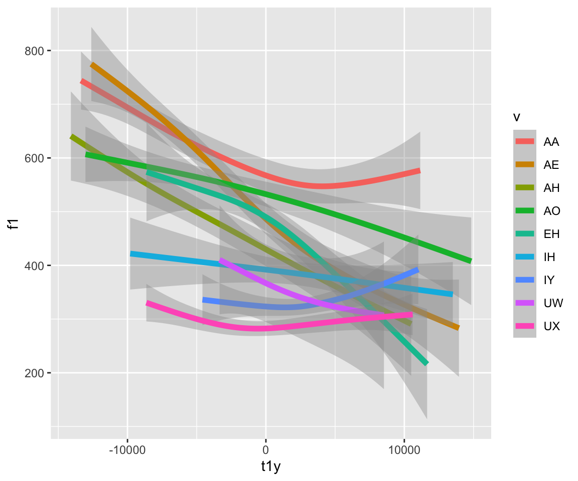
ggplot(ubdb, aes(x=t1y, y=f1)) + geom_line(aes(color = v))
ggplot(ubdb, aes(x=t1y, y=f1))+geom_ribbon(aes(color = v, ymin = f1-sd(f1), ymax = f1+sd(f1)), alpha = .2)+ geom_line(aes(color = v), size = 1.2)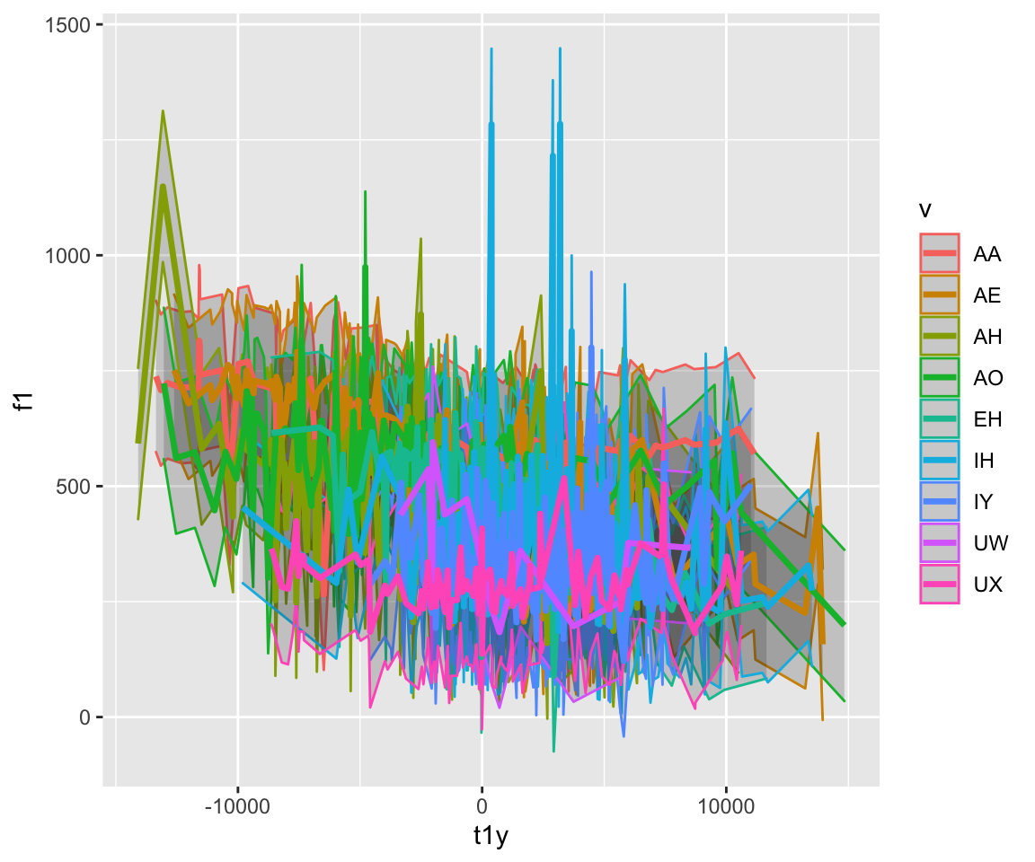
Other plots that we can do include using geom_text, geom_violin, and geom_bar, among many others!
ggplot(ubdb, aes(x=t1y, y=f1))+geom_text(aes(label=v, color = v))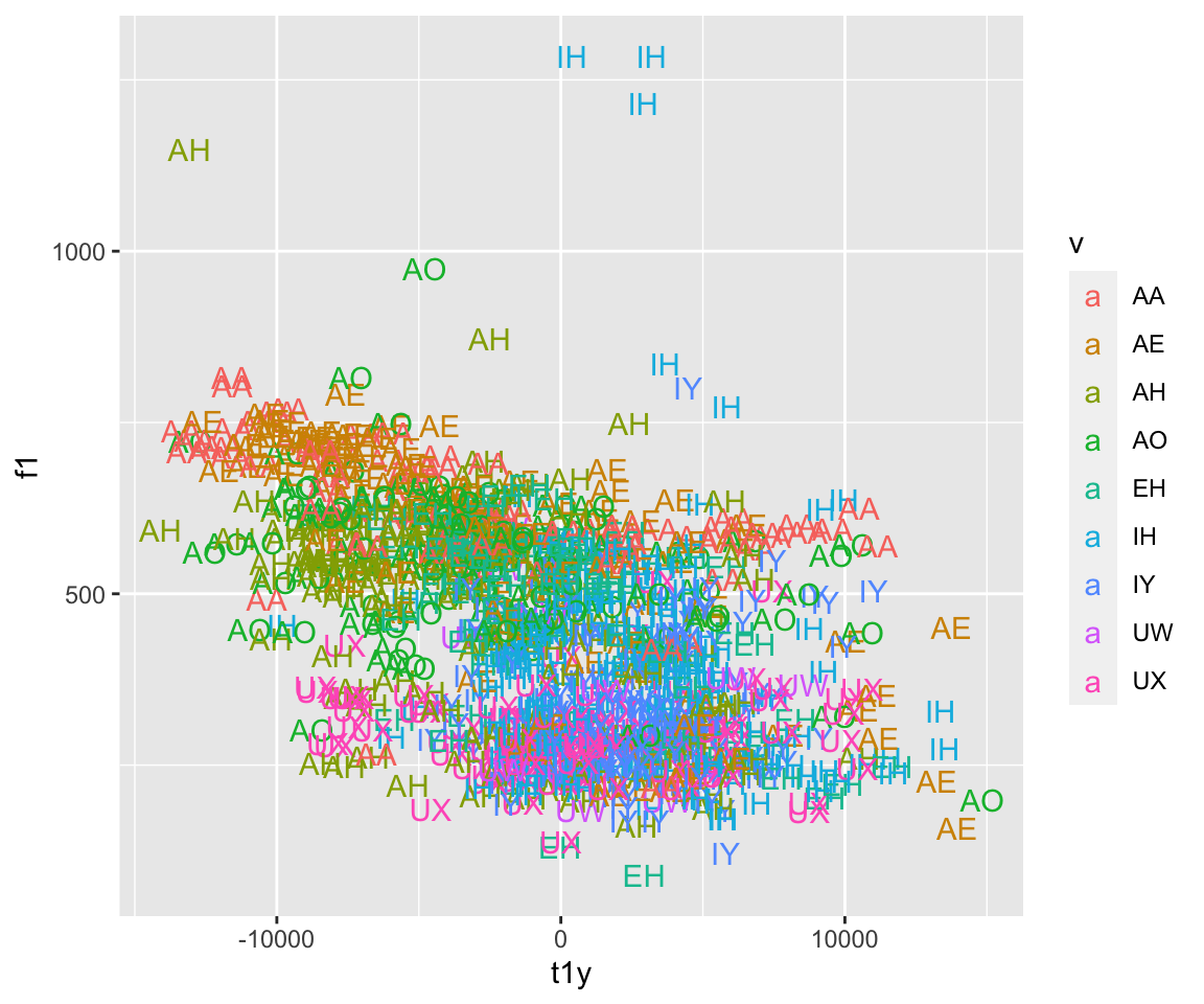
ggplot(ubdb, aes(x=v, y=f2))+geom_violin(aes(color = v))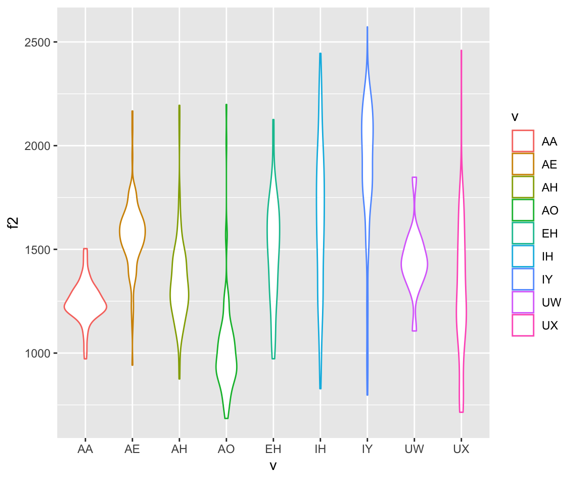
ggplot(ubdb, aes(x=v, y=f2))+geom_violin(aes(color = v, fill = v))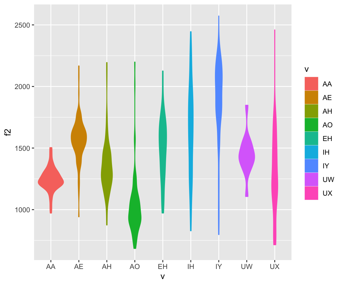
ggplot(ubdb, aes(x=v))+geom_bar(aes(color = v, fill = v))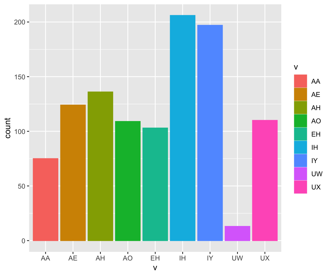
What if we wanted to plot the average F1 for each vowel? This doesn’t do it…
ggplot(ubdb, aes(x=v, y = f1))+geom_bar(aes(color = v, fill = v), stat = "identity")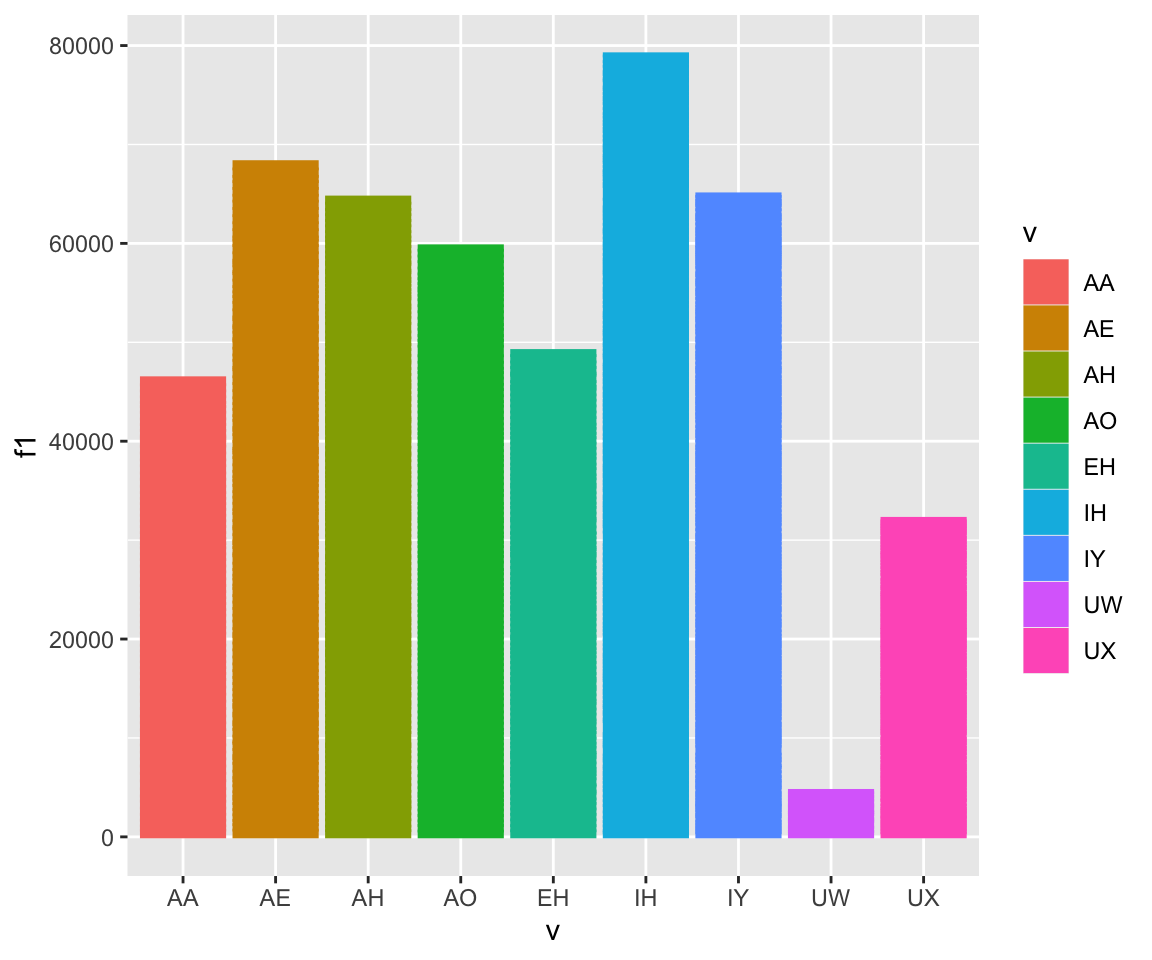 What we need to do is create a summary function and pass that into ggplot. This is a common thing to do for all sorts of data. In the summarise function, you can include standard error, SD, and many other summary statistics.
ubdbsummary = ubdb %>% group_by(v) %>% summarise(meanF1 = mean(f1), sdF1 = sd(f1))## `summarise()` ungrouping output (override with `.groups` argument)ggplot(ubdbsummary, aes(x=v, y = meanF1))+geom_bar(aes(color = v, fill = v), stat = "identity")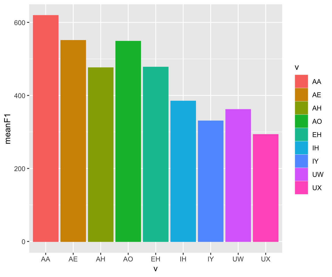
ggplot(ubdbsummary, aes(x=v, y = meanF1))+geom_bar(aes(color = v, fill = v), stat = "identity") + geom_errorbar(aes(ymin = meanF1-sdF1,ymax = meanF1+sdF1, group = v), width= 0.5)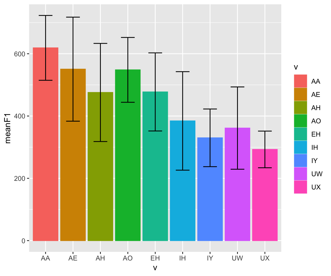
Faceting
Some of these graphs look pretty gross, because there is too much information on one single plot. A common way to deal with this is to do faceting, which splits the graph up into multiple graphs, based on one or more variable.
There are two functions that can be used to split the plots - facet_wrap() and facet_grid(). The first function, facet_wrap(), takes one grouping variable, splits the data up by that variable into multiple graphs, and then wraps the data into multiple rows. The variable being wrapped follows a tilde. The number of rows or columns can be specified (but not both!).
The second function, facet_grid(), takes two or more grouping variables, splits the data up by those variables into multiple graphs, and then wraps the data into multiple rows and columns based on the specified formula. Put the row-splitting variable(s) before the tilde, and the column-splitting variable(s) after the tilde. A period specifies no faceting along that dimension.
ggplot(ubdb, aes(x=t1y, fill=v)) + geom_density(size = 1, alpha=.2)+facet_wrap(~v)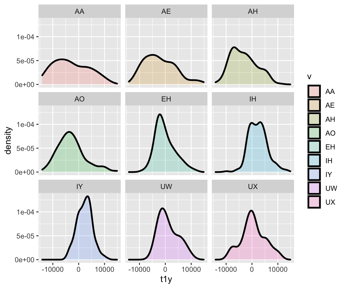
ggplot(ubdb, aes(x=t1y, y=f1)) + geom_point(aes(color = v), size = 2)+facet_grid(speaker~v)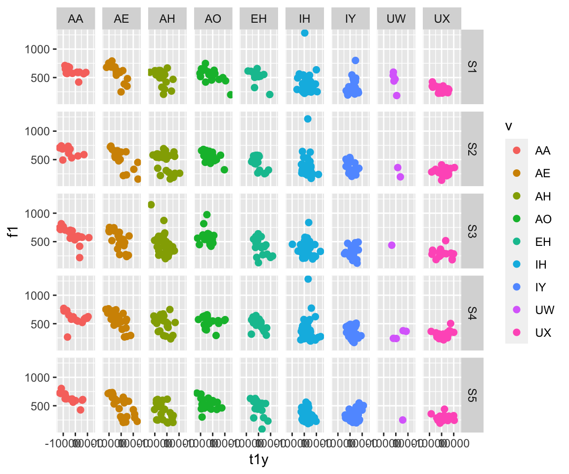
ggplot(ubdb, aes(x=t1y, y=f1)) + geom_point(aes(color = t4y), size = 2)+facet_grid(speaker~.)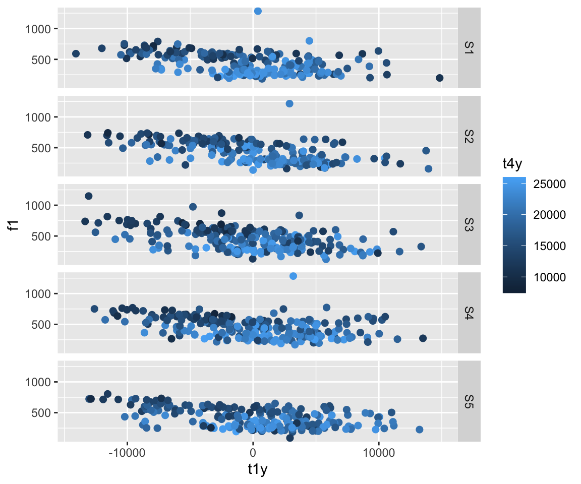
Statistical Transformations
So we’ve gone through various aesthetic calls for geometric objects. Note, however, that these objects are direct visualizations of the data, with no statistical transformations. What if we wanted to do something that showed statistical transforms? This could be helpful, as it would give summaries or more informative depictions of data, without the messiness of all of the points on the screen.
There are a few basic ones. First, you can do a histogram using stat_bin(). You can also use stat_summary(), which gives the mean and standard error of y at each x value (although other summary functions, such as median, mean and confidence interval, etc. can be used). stat_unique() removes duplicate values.
ggplot(ubdb, aes(x=t1y))+stat_bin()## `stat_bin()` using `bins = 30`. Pick better value with `binwidth`.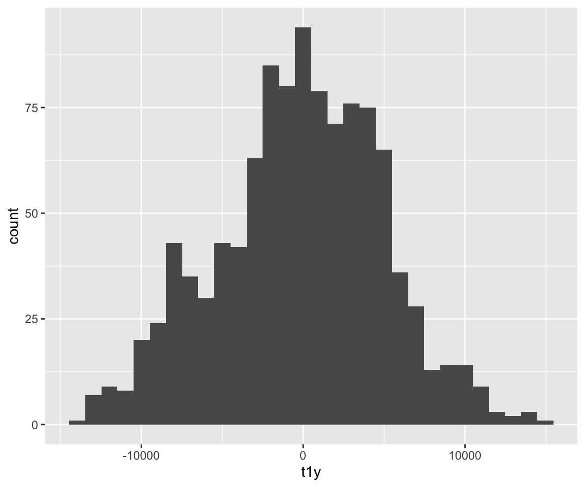
ggplot(ubdb, aes(x=t1y))+stat_bin(geom="point")## `stat_bin()` using `bins = 30`. Pick better value with `binwidth`.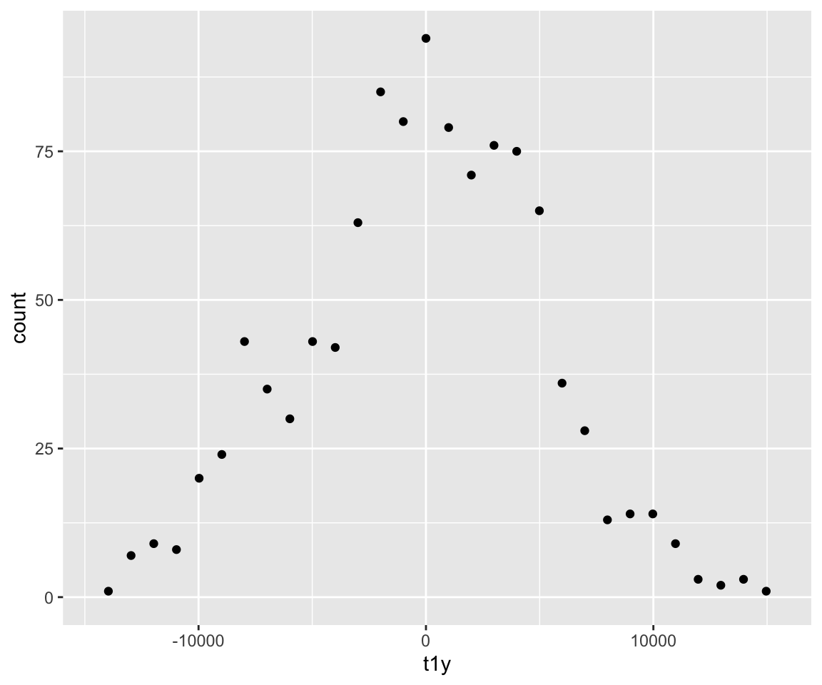
ggplot(ubdb, aes(x=t1y))+stat_bin(geom="line", bins = 50)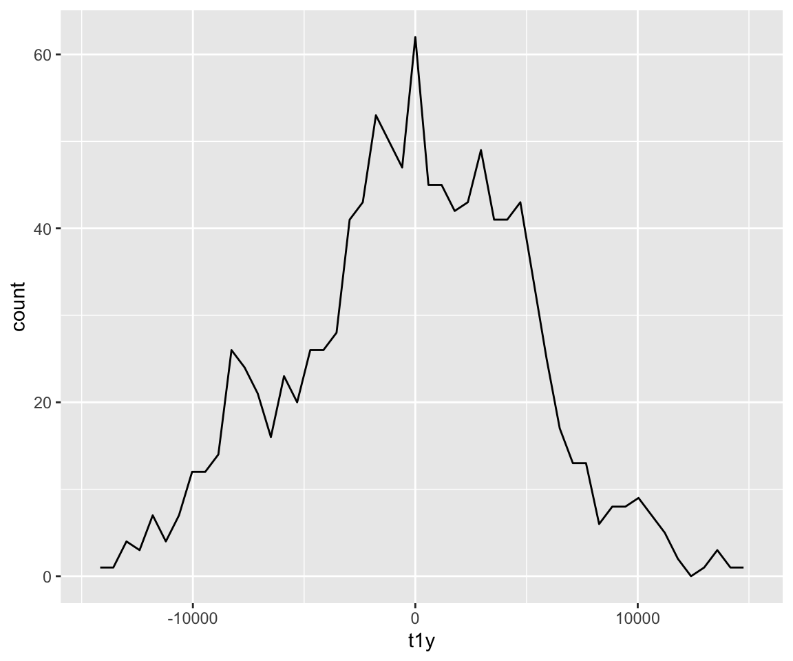
ggplot(ubdb, aes(x=t1y))+stat_bin(bins = 40)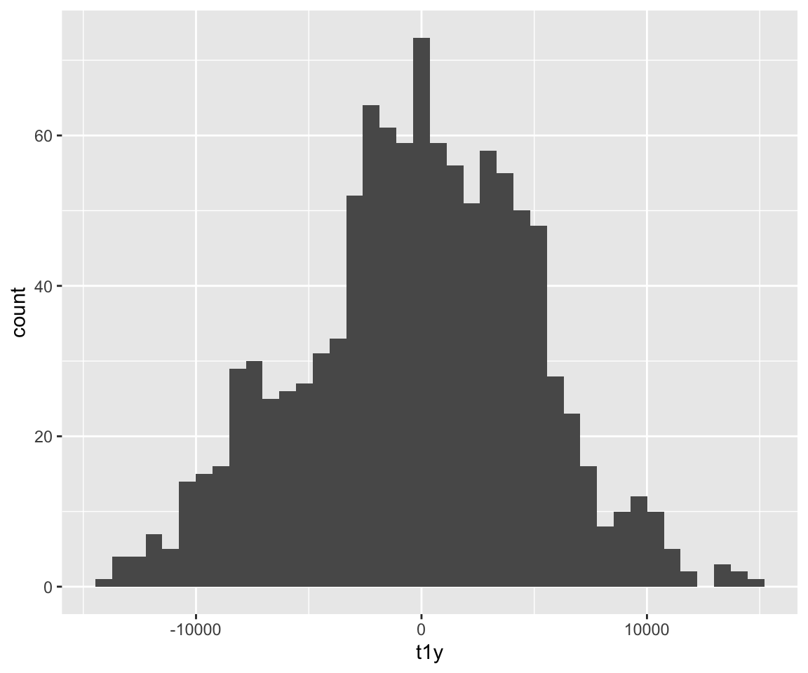
ggplot(ubdb, aes(x=v, y=t1y))+stat_summary()## No summary function supplied, defaulting to `mean_se()`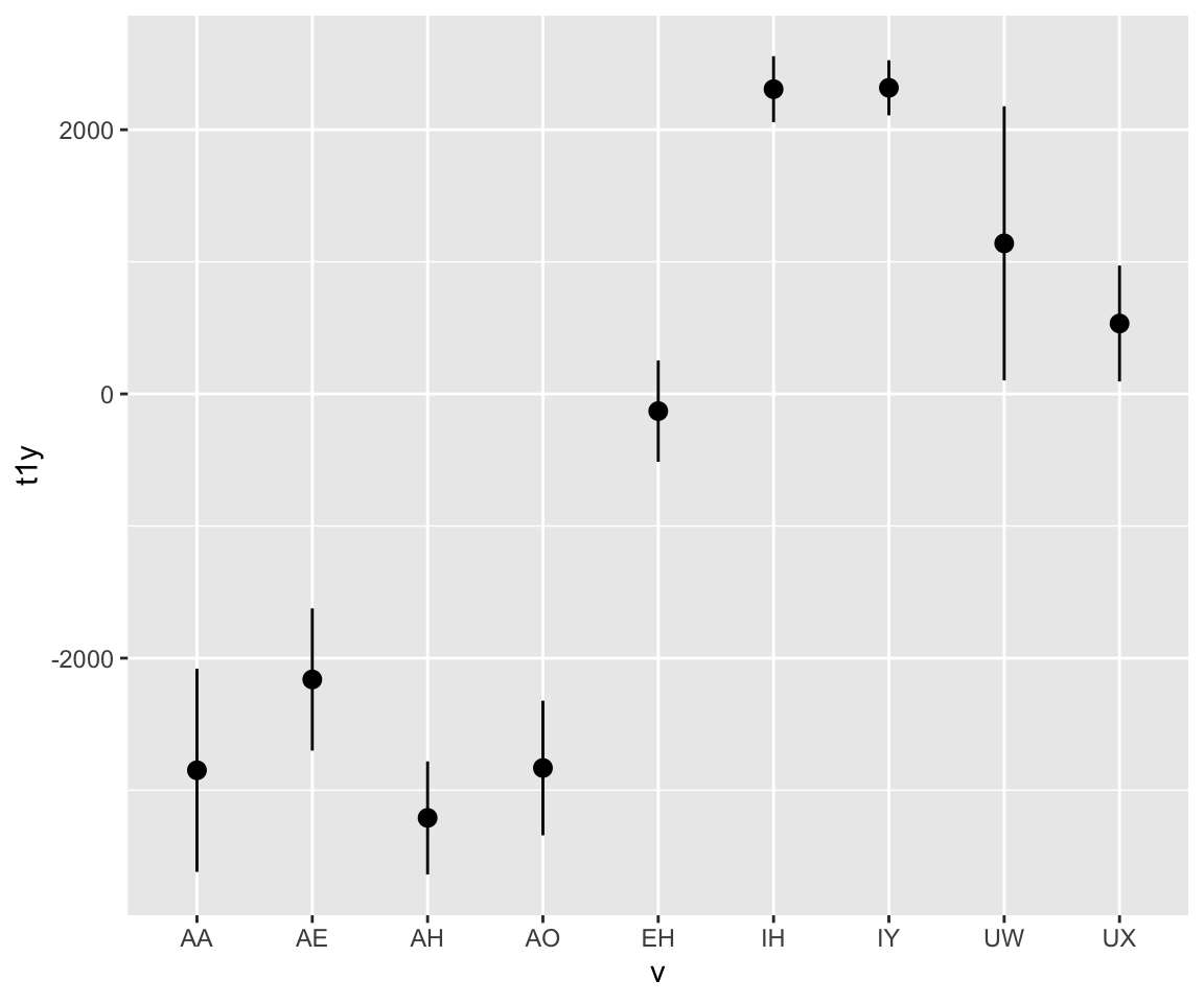
ggplot(ubdb, aes(x=t1y, y=f1)) + geom_point(aes(color = v)) + stat_unique()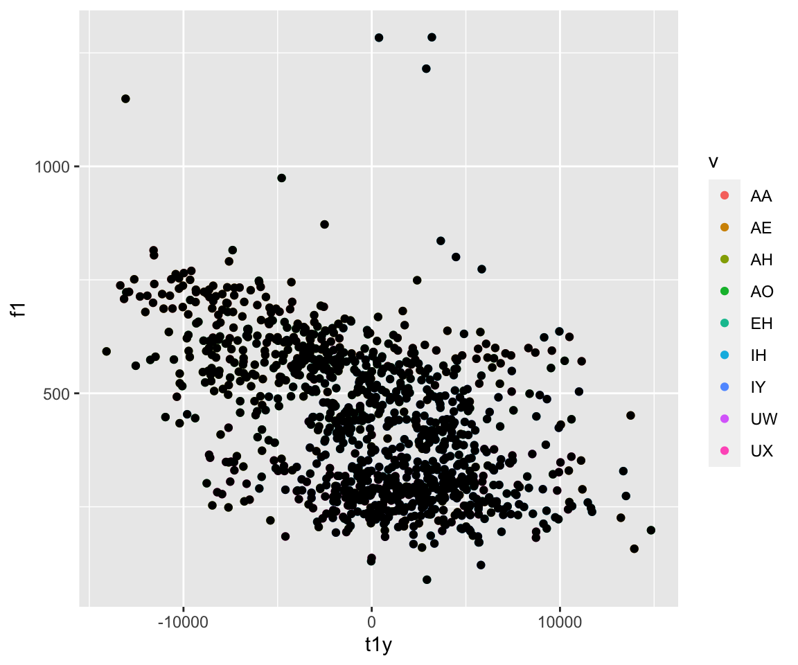
ggplot(ubdb, aes(x=f2, y=f1))+geom_point(aes(color = v))+stat_ellipse()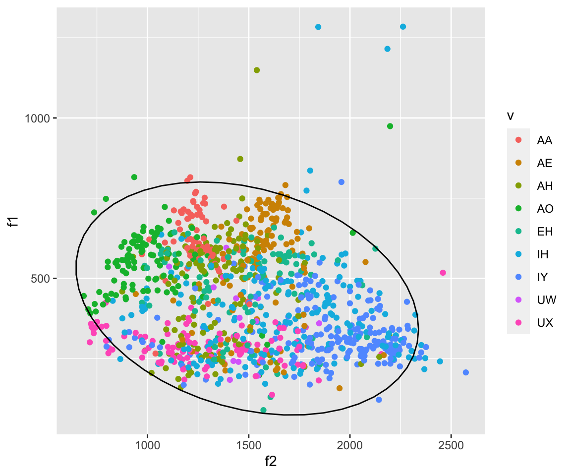
ggplot(ubdb, aes(x=f2, y=f1, color = v))+stat_ellipse(type = "norm")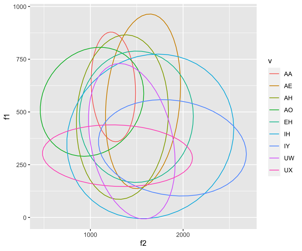
ggplot(ubdb, aes(x=f2, y=f1))+geom_point(aes(color = v))+stat_ellipse(aes(color = v))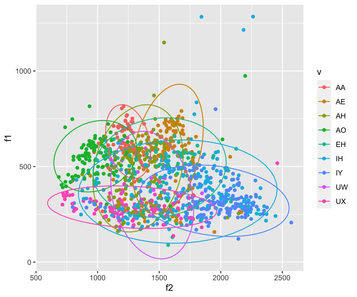
#Here I am breaking my own rule and using a second dataset, mymeans (which is the mean of F1 and F2 by vowel), in the plot to plot the centers of each ellipse.
mymeans = aggregate(ubdb[c("f1", "f2")], list(v=ubdb$v), mean)
mymeans2= aggregate(ubdb[c("f1", "f2")], list(v=ubdb$v, speaker = ubdb$speaker), mean)
ggplot(ubdb, aes(x=f2, y=f1))+geom_text(data = mymeans, aes(color = v, label = v), size = 4)+stat_ellipse(aes(color = v))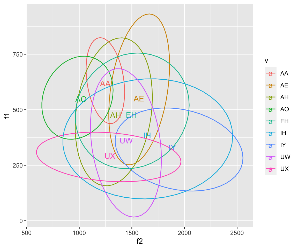
ggplot(ubdb, aes(x=f2, y=f1))+geom_text(data = mymeans, aes(color = v, label = v), size = 4)+stat_ellipse(aes(color = v, linetype = v))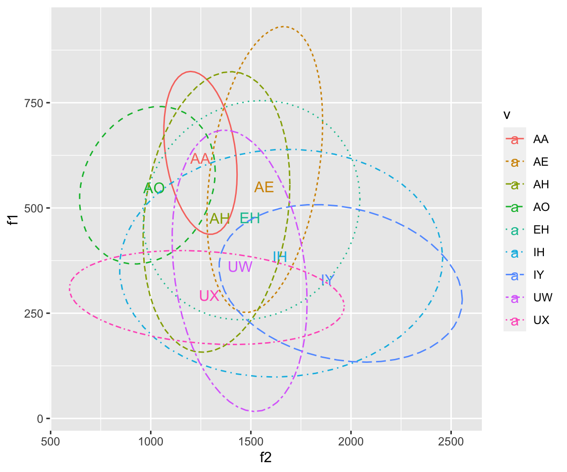
ggplot(ubdb, aes(x=f2, y=f1))+geom_text(data = mymeans, aes(color = v, label = v), size = 4)+stat_ellipse(aes(color = v, linetype = v))+ geom_point(aes(color = v), alpha = 0.2)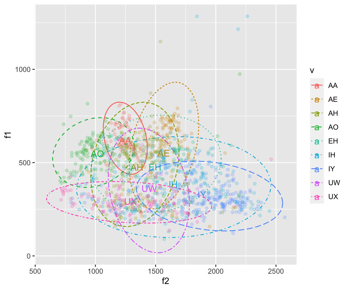
ggplot(ubdb, aes(x=f2, y=f1))+geom_text(data = mymeans2, aes(color = v, label = v), size = 4,show.legend = FALSE)+stat_ellipse(aes(color = v, linetype = v))+facet_wrap(~speaker)## Too few points to calculate an ellipse## Too few points to calculate an ellipse
## Too few points to calculate an ellipse## Warning: Removed 1 row(s) containing missing values (geom_path).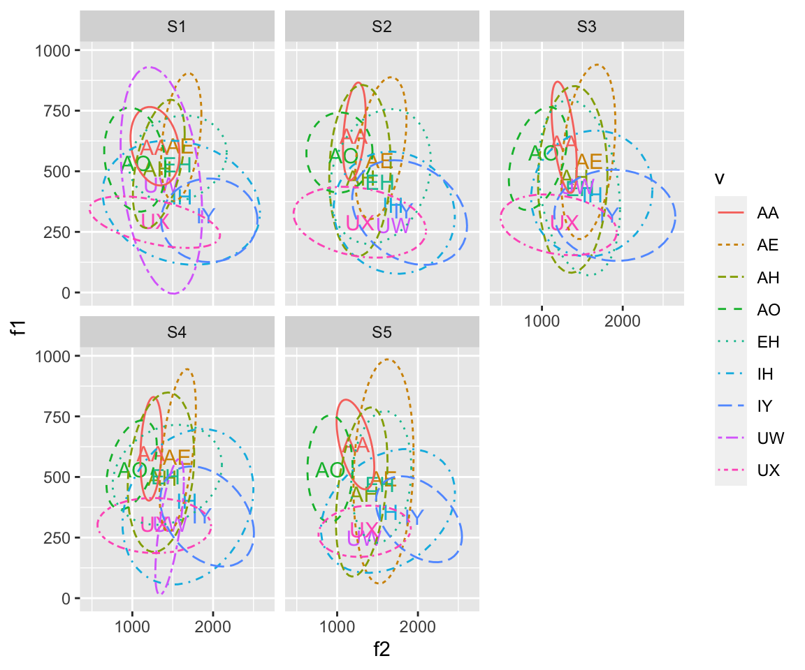
Other Aspects of the graph
Colors
There’s a lot to be said about different color palettes in R. You can specify your color scheme based on personal taste, school colors, using a colorblind friendly palette, etc. Note that it’s generally in good taste to use a colorblind friendly palette, which the base colors in ggplot are not, as they have the same luminescence. Below, I am defining a colorblind friendly palette and using it in graphs using scale_fill_manual() and scale_colour_manual(). You can do use these two functions with a predefined palette, as I am, or by calling color codes (either HTML or basic color names) in the function.
cbPalette <- c("#999999", "#E69F00", "#56B4E9", "#009E73", "#F0E442", "#0072B2", "#D55E00", "#CC79A7", "#000000")
cbPalette10= c("#543005", "#8c510a", "#bf812d", "#dfc27d", "#f6e8c3" ,"#c7eae5" ,"#80cdc1", "#35978f" ,"#01665e" ,"#003c30")
#To use for fills, add scale_fill_manual(values=cbPalette)
# To use for line and point colors, add scale_colour_manual(values=cbPalette)
ggplot(ubdb, aes(x=f2, y=f1))+geom_point(aes(color = v), alpha = 0.3)+stat_ellipse(aes(color = v))+scale_color_manual(values = cbPalette)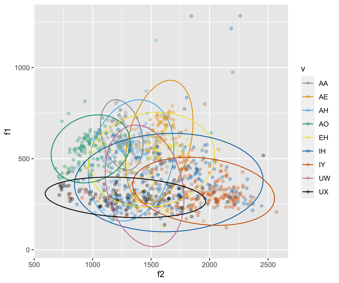 There are many other ways to define and change colors, including changing hues, luminance, saturation, etc. If you have any questions about these things, please ask me! You can also find more information on color in R here:
http://www.cookbook-r.com/Graphs/Colors_(ggplot2)/
###Labels, titles, and Axes If you want to relabel the axes, or give a title, you can use the xlab(), ylab(), and ggtitle() functions.
To change limits of the x and y axes, you can use xlim() and ylim().
You can reverse the order of the x and y axes using scale_x_reverse() and scale_y_reverse().
If you want to move the axes to the right/top, put these positions in the scale_x_continuous() and scale_y_continuous() functions. These can also go in the scale_x_reverse() and scale_y_reverse() functions. You can also specify two axes by calling for a second, duplicate axis. If you are using custom x and y scales and want to change the limits of the axes, do so inside of the scale functions calling limits = c(lim1, lim2). NOTE that if you are using scale_x_reverse() and/or scale_y_reverse() you have to include your limits in reverse!!
ggplot(ubdb, aes(x=f2, y=f1))+geom_point(aes(color = v))+stat_ellipse(aes(color = v))+scale_color_manual(values = cbPalette)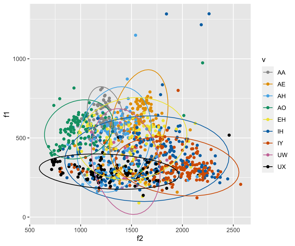
ggplot(ubdb, aes(x=f2, y=f1))+geom_point(aes(color = v))+stat_ellipse(aes(color = v))+scale_color_manual(values = cbPalette)+scale_x_reverse(position = "top")+scale_y_reverse(position = "right")+ xlab("F2!!!!") + ylab("F1!!!!!") + ggtitle("My vowel plot")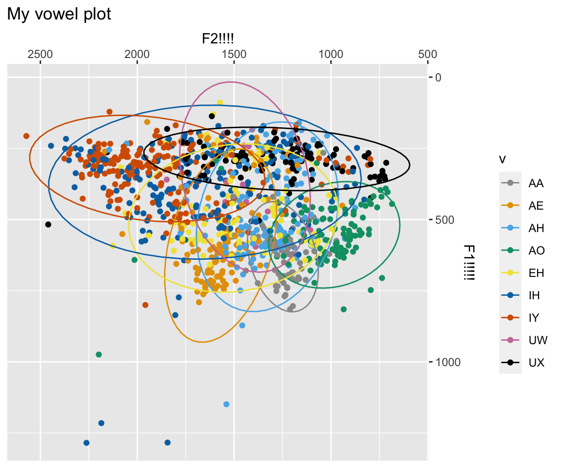
ggplot(ubdb, aes(x=f2, y=f1))+geom_point(aes(color = v))+stat_ellipse(aes(color = v))+scale_color_manual(values = cbPalette)+scale_x_reverse(position = "top", limits = c(2000,1000))+scale_y_reverse(position = "right", limits = c(2000,0))+ xlab("F2!!!!") + ylab("F1!!!!!") + ggtitle("My vowel plot")## Warning: Removed 236 rows containing non-finite values (stat_ellipse).## Warning: Removed 236 rows containing missing values (geom_point).## Warning: Removed 32 row(s) containing missing values (geom_path).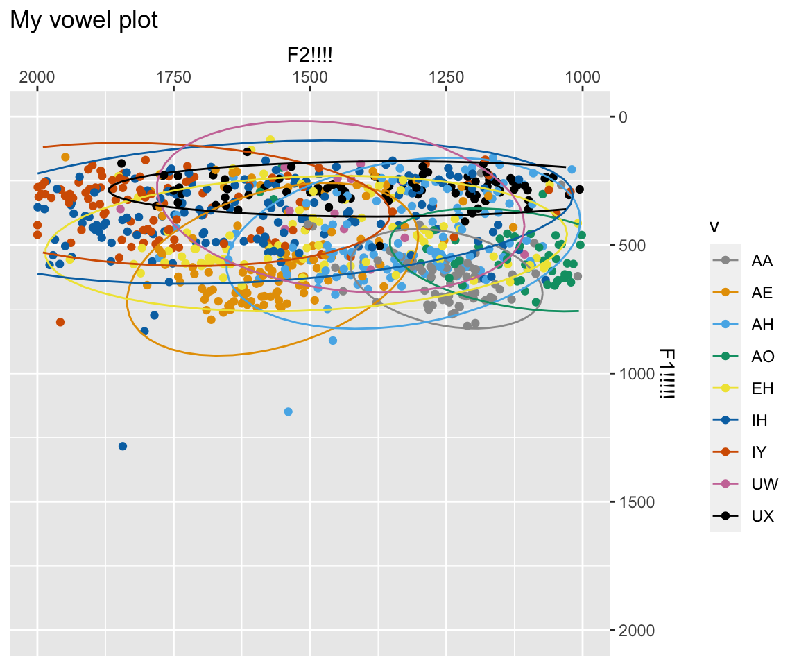
ggplot(ubdb, aes(x=f2, y=f1))+geom_point(aes(color = v))+stat_ellipse(aes(color = v))+scale_color_manual(values = cbPalette10, )+scale_x_reverse(sec.axis = dup_axis()) + scale_y_reverse(limits = (c(NULL,1500)),sec.axis = dup_axis())+ xlab("F2!!!!") + ylab("F1!!!!!") + ggtitle("My vowel plot")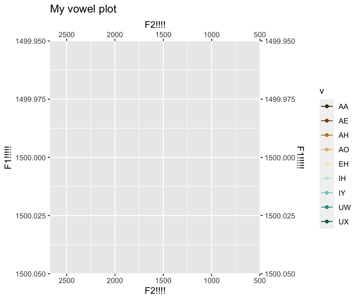
###Theme As you’ve noticed, there is a set theme about the graphs - the background is grey, the text is black, the gridlines are white, etc. There are a number of ways to change the theme around. The most common is to use a different complete theme, such as theme_minimal() or theme_grey(). You can also define your own theme settings.
ggplot(ubdb, aes(x=f2, y=f1))+geom_point(aes(color = v))+stat_ellipse(aes(color = v))+scale_color_manual(values = cbPalette)+scale_x_reverse(position = "top")+scale_y_reverse(position = "right")+ xlab("F2!!!!") + ylab("F1!!!!!") + ggtitle("My vowel plot") + theme_minimal()
ggplot(ubdb, aes(x=f2, y=f1))+geom_point(aes(color = v))+stat_ellipse(aes(color = v))+scale_color_manual(values = cbPalette)+scale_x_reverse(position = "top")+scale_y_reverse(position = "right")+ xlab("F2!!!!") + ylab("F1!!!!!") + ggtitle("My vowel plot") + theme(panel.grid.major = element_blank(),panel.grid.minor = element_blank(),panel.border = element_blank(), panel.background = element_blank())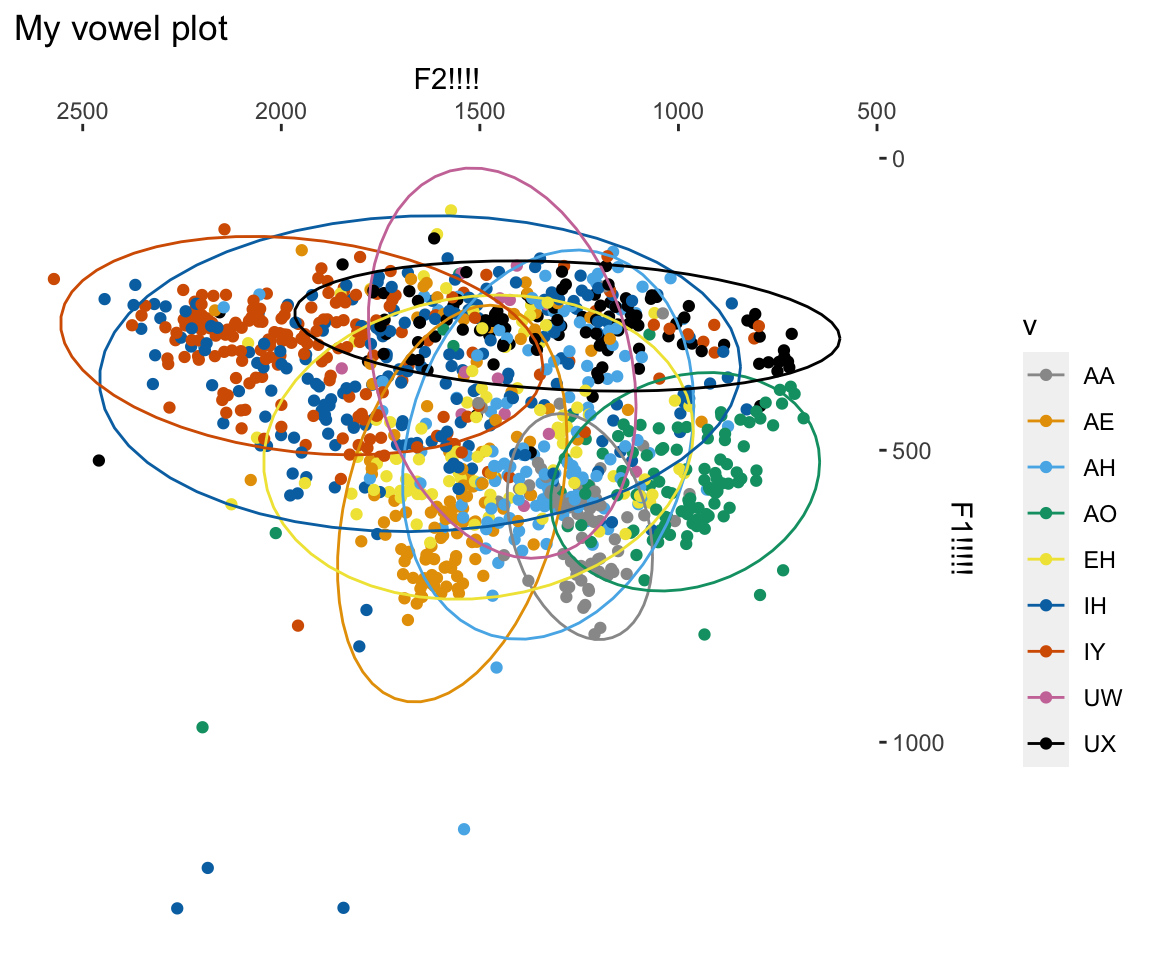
Wrapping up
In sum, ggplot2 is an extremely powerful package that can create lots of beautiful plots for your research. Think carefully about what you want to plot, and add layers as needed. I encourage you to save your plots as variables. You can then view and save them.
myplot = ggplot(ubdb, aes(x=f2, y=f1))+geom_point(aes(color = v), alpha = 0.2, size = 0.4)+stat_ellipse(aes(color = v))+scale_color_manual(values = cbPalette)+scale_x_reverse(position = "top")+scale_y_reverse(position = "right")+ xlab("F2!!!!") + ylab("F1!!!!!") + ggtitle("My vowel plot") + theme_minimal() + geom_label(data = mymeans,aes(color = v, label = v), size = 4,show.legend =FALSE)

myplot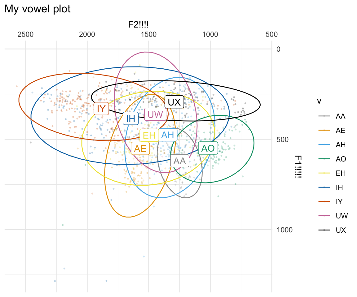
#Not run = to save the plot!
#ggsave("myplot.pdf", plot = myplot, height = 6, width = 10, units = "in", device = cairo_pdf)
I highly recommend using the following reference whenever you need to find more information about a graphing mechanism in ggplot: http://ggplot2.tidyverse.org/reference/