Phonetics Tools in R
library(tidyverse)## ── Attaching packages ────────────────────────────────────────────────────────────── tidyverse 1.3.0 ──## ✓ ggplot2 3.3.2 ✓ purrr 0.3.4
## ✓ tibble 3.0.3 ✓ dplyr 1.0.2
## ✓ tidyr 1.1.2 ✓ stringr 1.4.0
## ✓ readr 1.3.1 ✓ forcats 0.5.0## ── Conflicts ───────────────────────────────────────────────────────────────── tidyverse_conflicts() ──
## x dplyr::filter() masks stats::filter()
## x dplyr::lag() masks stats::lag()library(PraatR)
library(rPraat)
library(phonR)
library(dygraphs)
library(phonTools)##
## Attaching package: 'phonTools'## The following object is masked from 'package:dplyr':
##
## slicelibrary(audio)##
## Attaching package: 'audio'## The following object is masked from 'package:phonTools':
##
## playlibrary(tuneR)##
## Attaching package: 'tuneR'## The following object is masked from 'package:audio':
##
## play## The following objects are masked from 'package:phonTools':
##
## normalize, playlibrary(gss)For this workshop, I will be using a subset of my dissertation data. I will be using words with oral vowels in Brazilian Portuguese (/a/ from the word babado, /i/ from the word cabido, and /u/ from the word tributo), repeated by five female speakers in a carrier phrase. The audio files and accompanying textgrids I use are named as follows:
absdir = "/Users/marissabarlaz/Desktop/FemaleBP/"
mydir = list.files(absdir, "*.WAV")
mydir
## [1] "BP17-L-babado.WAV" "BP17-L-cabido.WAV" "BP17-L-tributo.WAV"
## [4] "BP18-L-babado.WAV" "BP18-L-cabido.WAV" "BP18-L-tributo.WAV"
## [7] "BP19-L-babado.WAV" "BP19-L-cabido.WAV" "BP19-L-tributo.WAV"
## [10] "BP20-L-babado.WAV" "BP20-L-cabido.WAV" "BP20-L-tributo.WAV"
## [13] "BP21-L-babado.WAV" "BP21-L-cabido.WAV" "BP21-L-tributo.WAV"testwav = paste0(absdir, mydir[1])
testwav## [1] "/Users/marissabarlaz/Desktop/FemaleBP/BP17-L-babado.WAV"testtext = str_replace(testwav, ".WAV", ".TextGrid")
testformant = str_replace(testwav, ".WAV", ".Formant")
testpitch = str_replace(testwav, ".WAV", ".Pitch")
testpitchtier = str_replace(testwav, ".WAV", ".PitchTier")
testint = str_replace(testwav, ".WAV", ".Intensity")
testinttier = str_replace(testwav, ".WAV", ".IntensityTier")
testtable = str_replace(testwav, ".WAV", ".Table")For these analyses, I will be using text grids I have already created. It is possible to do annotations with R, but it can be very time consuming, and involves knowing the exact start and end points of sounds.
The audio files can be found here.
PraatR
First, we will talk about how to actually call Praat from R using the praatR package.
Before you begin, it is important to figure out what settings you will want for formant analysis, and pitch analysis.
FormantArguments = list( 0.001, # Time step (s)
                         5,     # Max. number of formants
                         5500,  # Maximum formant (Hz)
                         0.025, # Window length (s)
                         50    )# Pre-emphasis from (Hz)

PitchArguments = list( 0.001,   # Time step (s)
                       75,      # Pitch floor
                       350 )    # Pitch ceiling
Pitch analysis
Basically, PraatR works by creating new .Pitch, .PitchTier, etc. files. You use the praat() function to call any sort of function you would use in R. Note that this package is extremely finnicky about spaces in names of folders/paths.
praat( "To Pitch...", arguments=PitchArguments, input=testwav, output=testpitch, overwrite=TRUE )
praat( "Down to PitchTier", input=testpitch, output=testpitchtier, overwrite=TRUE, filetype="headerless spreadsheet" )
PitchTierData = read.table(testpitchtier, col.names=c("Time","F0"))
head(PitchTierData)
## Time F0
## 1 0.02016667 260.6060
## 2 0.02116667 260.3456
## 3 0.02216667 260.1420
## 4 0.02316667 259.9835
## 5 0.02416667 259.8604
## 6 0.02516667 259.7627praat( "Down to Table...",
arguments = list( FALSE, # Include line number
10, # Time decimals
TRUE, # Include tier names
FALSE # Include empty intervals
), # End list()
input=testtext,
output=testtable,
filetype="tab-separated",
overwrite = TRUE
)
TextGridTable = read.delim(testtable)
head(TextGridTable)## tmin tier text tmax
## 1 0.3685511 segment ao 0.5662138
## 2 3.5062709 segment ao 3.6929523
## 3 6.0017163 segment ao 6.1883977
## 4 8.5326568 segment ao 8.7229987
## 5 11.0302097 segment ao 11.2315328
## 6 13.5066505 segment ao 13.6915017What if you wanted to get the pitch for each particular sound, let’s say at their midpoints?
TextGridTable = TextGridTable %>% mutate(midpoint = (tmax + tmin)/2)
praat( "Get value at time...", arguments=list(TextGridTable$midpoint[5], "Hertz", "Linear"), input=testpitch)
## [1] "206.1084180844884 Hz"#Loop
for (i in 1:length(TextGridTable$midpoint)){
TextGridTable$F0_mdpt[i] = praat( "Get value at time...", arguments=list(TextGridTable$midpoint[i], "Hertz", "Linear"), input=testpitch)
}
#sapply(TextGridTable$midpoint, function(x) praat( "Get value at time...", arguments=list(x, "Hertz", "Linear"), input=testpitch))
head(TextGridTable)## tmin tier text tmax midpoint F0_mdpt
## 1 0.3685511 segment ao 0.5662138 0.4673824 206.13880905863698 Hz
## 2 3.5062709 segment ao 3.6929523 3.5996116 199.87076326158552 Hz
## 3 6.0017163 segment ao 6.1883977 6.0950570 202.56410033498975 Hz
## 4 8.5326568 segment ao 8.7229987 8.6278278 199.7400301550135 Hz
## 5 11.0302097 segment ao 11.2315328 11.1308712 206.1084180844884 Hz
## 6 13.5066505 segment ao 13.6915017 13.5990761 206.74855943457132 HzNow, what if you wanted to get 5 points of time?
TextGridTable = TextGridTable %>% group_by(tmin) %>%
  mutate(timept = list(seq(1,5,1)),
         fivepts= list(seq(from = tmin, to = tmax, by = (tmax-tmin)/4))) %>%
  unnest()

#This doesn't work - use a for loop instead, or sapply as above
#TextGridTable %>% mutate(
#F0 = praat( "Get value at time...", arguments=list(fivepts, "Hertz", "Linear"), input = testpitch))

TextGridTable$F0= 0
for (i in 1:length(TextGridTable$fivepts)){
  TextGridTable$F0[i] = praat( "Get value at time...", arguments=list(TextGridTable$fivepts[i], "Hertz", "Linear"), input=testpitch)
  }
Now, your formant outputs are character class. In order to change this to numeric, we will first remove ‘Hz’ from the character, then convert to numeric. Anything that is ‘undefined’ will be turned into an NA.
TextGridTable = TextGridTable %>% mutate_at(.vars = c("F0_mdpt", "F0"), .funs = str_replace_all, pattern = "Hz", replacement = "") %>% mutate_at(.vars = c("F0_mdpt", "F0"), .funs = str_replace_all, pattern = "--undefined--", replacement = "NA") %>% mutate_at(.vars = c("F0_mdpt", "F0"), .funs = as.numeric)OK, so that was done for one file. What about for multiple files? We need to put this all into a loop.
starttime = Sys.time()
alltextgrids = list()
for (j in 1:length(mydir)){
curwav = paste0(absdir, mydir[j])
curtext = str_replace(curwav, ".WAV", ".TextGrid")
curpitch = str_replace(curwav, ".WAV", ".Pitch")
curpitchtier = str_replace(curwav, ".WAV", ".PitchTier")
curtable = str_replace(curwav, ".WAV", ".Table")

#createtextgrid
praat( "Down to Table...",
       arguments = list( FALSE, # Include line number
                         10,    # Time decimals
                         TRUE, # Include tier names
                         FALSE  # Include empty intervals
                       ), # End list()
       input=curtext,
       output=curtable,
       filetype="tab-separated",
       overwrite = TRUE

       ) # End call to 'praat()'

TextGridTable = read.delim(curtable)
TextGridTable$Speaker = substr(mydir[1], 1, 4)
TextGridTable = TextGridTable %>% mutate(RepNo = as.numeric(as.factor(tmin)))%>% group_by(tmin) %>%
  mutate(normtime = list(seq(0.1,1.0,.1)),
         acttimenorm= list(seq(from = tmin, to = tmax, by = (tmax-tmin)/9))) %>%
  unnest()

praat( "To Pitch...", arguments=PitchArguments, input=curwav, output=curpitch, overwrite=TRUE )
for (i in 1:length(TextGridTable$acttimenorm)){
  TextGridTable$F0[i] = praat( "Get value at time...", arguments=list(TextGridTable$acttimenorm[i], "Hertz", "Linear"), input=curpitch)
  }
TextGridTable = TextGridTable %>% mutate(F0 = as.numeric(str_replace_all(str_replace_all(F0, pattern = "Hz", replacement = ""), pattern = "--undefined--", replacement = "NA")))

alltextgrids[[j]] = TextGridTable
#file.remove(c(curpitch, curtable))
rm(TextGridTable, curwav, curtable, curpitch, curtext, curpitchtier)
}

all_f0_data_PraatR <- do.call("rbind", alltextgrids) %>% select(tmin, tmax, text, Speaker, RepNo, normtime, acttimenorm, F0) %>% rename(label = text)
rm(alltextgrids, i, j)
endtime = Sys.time()
endtime - starttime
## Time difference of 1.40635 hoursYou can also do things like formant analysis the same way. I will not go through the entirety of a for loop, but just will show you an example on the testwav file I used before.
FormantTable = read.delim(testtable)
praat( "To Formant (burg)...",arguments = FormantArguments,input = testwav, output = testformant, overwrite = TRUE) # End praat()

FormantTable = FormantTable %>% mutate(midpoint = (tmax + tmin)/2, F1_mdpt = 0, F2_mdpt = 0, F3_mdpt = 0)

for (i in 1:length(FormantTable$midpoint)){
  FormantTable$F1_mdpt[i] = praat( "Get value at time...", arguments=list(1, FormantTable$midpoint[i], "Hertz", "Linear"), input=testformant)
  FormantTable$F2_mdpt[i] = praat( "Get value at time...", arguments=list(2, FormantTable$midpoint[i], "Hertz", "Linear"), input=testformant)
  FormantTable$F3_mdpt[i] = praat( "Get value at time...", arguments=list(3, FormantTable$midpoint[i], "Hertz", "Linear"), input=testformant)
  }

head(FormantTable)
## tmin tier text tmax midpoint F1_mdpt
## 1 0.3685511 segment ao 0.5662138 0.4673824 883.2807619506391 hertz
## 2 3.5062709 segment ao 3.6929523 3.5996116 921.21054130018 hertz
## 3 6.0017163 segment ao 6.1883977 6.0950570 891.476628700663 hertz
## 4 8.5326568 segment ao 8.7229987 8.6278278 894.5945631724654 hertz
## 5 11.0302097 segment ao 11.2315328 11.1308712 951.6006078560181 hertz
## 6 13.5066505 segment ao 13.6915017 13.5990761 922.6018852827742 hertz
## F2_mdpt F3_mdpt
## 1 1541.2145741840059 hertz 3076.798429305465 hertz
## 2 1570.7125874327346 hertz 3048.6353438460546 hertz
## 3 1601.201093375497 hertz 3002.8616503410567 hertz
## 4 1572.5047603271003 hertz 2994.0426186571212 hertz
## 5 1585.5962991072736 hertz 3057.4259220868607 hertz
## 6 1401.9751550767953 hertz 3050.813680335225 hertzFormantTable = FormantTable %>% mutate_at(.vars = c("F1_mdpt", "F2_mdpt", "F3_mdpt"), .funs = str_replace_all, pattern = "hertz", replacement = "") %>% mutate_at(.vars = c("F1_mdpt", "F2_mdpt", "F3_mdpt"), .funs = str_replace_all, pattern = "--undefined--", replacement = "NA") %>% mutate_at(.vars = c("F1_mdpt", "F2_mdpt", "F3_mdpt"), .funs = as.numeric)All commands supported in the PraatR package are listed here.
rPraat
PraatR takes a really long time to run. A really long time. rPraat also can take a while, but is good for doing Praat-related inquiries R-internally, rather than interfacing with Praat. It once again takes things already made in Praat as inputs, such as PitchTier and IntensityTier. Here, I will use the PraatR functions in order to create these, rather than opening R.
Using rPraat, you can also create interactive graphs, called dygraphs. You can do them for textgrids, pitch tiers, and intensity tiers, but right now there is not a way to do it together, except by hacking together a plot.
praat( "To Pitch...", arguments=PitchArguments, input=testwav, output=testpitch, overwrite=TRUE )
praat( "Down to PitchTier", input=testpitch, output=testpitchtier, overwrite=TRUE, filetype="headerless spreadsheet" )

praat( "To Intensity...", arguments = list(100, 0), input=testwav, output=testint, overwrite=TRUE )
praat( "Down to IntensityTier", input=testint, output=testinttier, overwrite=TRUE, filetype="text" )


tg.test = tg.read(testtext)
pt.test = pt.read(testpitchtier)
it.test = it.read(testinttier)
#Plot individually using groups
tg.plot(tg.test, group = "testplot")
pt.plot(pt.test, group = "testplot")
it.plot(it.test, group = "testplot")
#plot sound
sndWav <- readWave(testwav); fs <- sndWav@samp.rate; snd <- sndWav@left / (2^(sndWav@bit-1))
t <- seqM(0, (length(snd)-1)/fs, by = 1/fs)
dygraph(data.frame(t, snd), xlab = "Time (sec)", group = "testplot")%>% dyRangeSelector(height = 20)
rm(sndWav, t)Using apply to create .Pitch files
Things I didn’t know when I started writing this workshop - you CAN use apply functions to create all .Pitch and .PitchTier, etc. files on your computer. Once again, use absolute paths without spaces in them! This will make your life a lot easier, though sadly it does NOT make things shorter in terms of time.
mydirlong = "/Users/marissabarlaz/Desktop/FemaleBP/"
mydirwav = paste0(mydirlong, mydir)
mydirpitch = str_replace_all(mydirwav, ".WAV", ".Pitch")
mydirpitchtier = str_replace_all(mydirwav, ".WAV", ".PitchTier")
mydirall = cbind(mydirwav, mydirpitch, mydirpitchtier)

#lapply(seq(1,dim(mydirall)[1],1), function(x) praat( "To Pitch...", arguments=PitchArguments, input=mydirall[x,1], output=mydirall[x,2], overwrite=TRUE ))

#OR!


apply(mydirall,1, function(x) praat( "To Pitch...", arguments=PitchArguments, input=x[1], output=x[2], overwrite=TRUE ))
## NULLWhat if we wanted to get the midpoint of pitch for each vowel in the textgrid?
tg.ao = tg.findLabels(tg.test, 1, labelVector = c("ao"), returnTime = TRUE)
tg = data.frame(t1 =tg.test$segment$t1, t2 = tg.test$segment$t2, label = tg.test$segment$label) %>% filter(label =="ao") %>% mutate(f0_mdpt = 0)


for (i in 1:length(tg.ao$t1)){
  mdpt = (tg$t1[i] + tg$t2[i])/2
  mywhichmdpt = which.min(abs(mdpt -pt.test$t))
    tg$f0_mdpt[i] = pt.test$f[mywhichmdpt]
}

head(tg)
## t1 t2 label f0_mdpt
## 1 0.3685511 0.5662138 ao 206.1531
## 2 3.5062709 3.6929523 ao 199.9026
## 3 6.0017163 6.1883977 ao 202.5589
## 4 8.5326568 8.7229987 ao 199.7170
## 5 11.0302097 11.2315328 ao 206.0849
## 6 13.5066505 13.6915017 ao 206.7488Now, what if we wanted to get pitch information for 10 points throughout vowel duration, like we did before? Let’s put this all in a loop. Before, I did not delete the Pitch information off of my computer, so I am using that as a starting point.
starttime2 = Sys.time()
alltextgrids2 = list()
for (j in 1:length(mydir)){
  curwav = paste0(absdir, mydir[j])
curtext = str_replace(curwav, ".WAV", ".TextGrid")
curpitch = str_replace(curwav, ".WAV", ".Pitch")
curpitchtier = str_replace(curwav, ".WAV", ".PitchTier")
curtable = str_replace(curwav, ".WAV", ".Table")

TextGridInfo = tg.read(curtext)
CurTextGrid = data.frame(tmin =TextGridInfo$segment$t1, tmax = TextGridInfo$segment$t2, label = TextGridInfo$segment$label) %>% filter(label !="")
CurTextGrid$Speaker = substr(mydir[1], 1, 4)
CurTextGrid = CurTextGrid %>% mutate(RepNo = as.numeric(as.factor(tmin))) %>% group_by(tmin) %>%
  mutate(normtime = list(seq(0.1,1.0,.1)),
         acttimenorm= list(seq(from = tmin, to = tmax, by = (tmax-tmin)/9))) %>%
  unnest()

praat( "Down to PitchTier", input=curpitch, output=curpitchtier, overwrite=TRUE, filetype="headerless spreadsheet" )
PitchTierInfo = pt.read(curpitchtier)

for (k in 1:length(CurTextGrid$acttimenorm)){

mytime = CurTextGrid$acttimenorm[k]
    mywhichpt = which.min(abs(mytime - PitchTierInfo$t))
    CurTextGrid$F0[k] = PitchTierInfo$f[mywhichpt]
  }

alltextgrids2[[j]] = CurTextGrid
#file.remove(c(curpitch, curtable))
rm(CurTextGrid, curwav, curtable, curpitch, curtext, curpitchtier)
}

all_f0_data_rPraat <- do.call("rbind", alltextgrids2)
head(all_f0_data_rPraat)
## # A tibble: 6 x 8
## # Groups: tmin [1]
## tmin tmax label Speaker RepNo normtime acttimenorm F0
## <dbl> <dbl> <chr> <chr> <dbl> <dbl> <dbl> <dbl>
## 1 0.369 0.566 ao BP17 1 0.1 0.369 204.
## 2 0.369 0.566 ao BP17 1 0.2 0.391 210.
## 3 0.369 0.566 ao BP17 1 0.3 0.412 211.
## 4 0.369 0.566 ao BP17 1 0.4 0.434 209.
## 5 0.369 0.566 ao BP17 1 0.5 0.456 207.
## 6 0.369 0.566 ao BP17 1 0.6 0.478 205.rm(alltextgrids, i, j)
endtime2 = Sys.time()
endtime2 - starttime2## Time difference of 43.96095 secsUnfortunately, as of now, we cannot do formant analysis with rPraat. You can do intensity analysis, if you would like.
PhonTools
PhonTools uses a lot of methods similar to what Praat uses, but it doesn’t use Praat objects. All calculations of formants and f0 are internal to R. Analyses rely heavily on the audio and tuneR packages.
Pitch tracking
Here, I reading in an audio file and a textgrid, creating a pitch track, and getting F0 at the midpoint of vowels. Because PhonTools doesn’t interact with Praat, you have to use a PraatR or RPraat function to import TextGrids, or use rjson. I will show you how to do it with both.
sndWav <- readWave(testwav); fs <- sndWav@samp.rate; snd <- sndWav@left / (2^(sndWav@bit-1))
t <- seqM(0, (length(snd)-1)/fs, by = 1/fs)

sound = makesound((sndWav@left / (2^(sndWav@bit-1))), mydir[1], fs = sndWav@samp.rate)
mytrack = formanttrack(sound, show = FALSE)

mypitch = pitchtrack(sound, f0range = c(60,400), timestep = 2, minacf = .5,correction = TRUE, show = TRUE, windowlength = 50, addtospect = FALSE)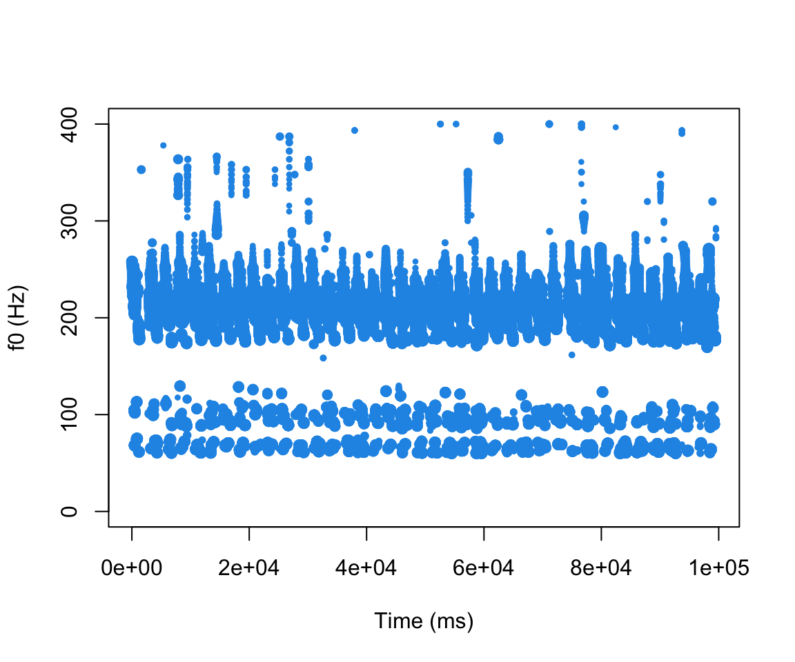
mypitch$time = mypitch$time/1000

#using PraatR
mytable = read.delim(testtable) %>% mutate(midpoint = (tmin+tmax)/2)

mytable$f0_mdpt = mypitch$f0[sapply(mytable$midpoint,function(x) which.min(abs(x-mypitch$time)))]
I personally like using RPraat better, because you don’t need to use a Praat command to create a Table. Rather, you transform the textgrid into a dataframe right in R.
starttime3 = Sys.time()
alltextgrids3 = list()
for (j in 1:length(mydir)){
curwav = paste0(absdir, mydir[j])
curtext = str_replace(curwav, ".WAV", ".TextGrid")

#Using RPraat
TextGridInfo = tg.read(curtext)
CurTextGrid = data.frame(tmin =TextGridInfo$segment$t1, tmax = TextGridInfo$segment$t2, label = TextGridInfo$segment$label) %>% filter(label !="")
CurTextGrid$Speaker = substr(mydir[1], 1, 4)
CurTextGrid = CurTextGrid %>% mutate(RepNo = as.numeric(as.factor(tmin))) %>%  group_by(tmin) %>%
  mutate(normtime = list(seq(0.1,1.0,.1)),
         acttimenorm= list(seq(from = tmin, to = tmax, by = (tmax-tmin)/9))) %>%
  unnest()


CurAudio = readWave(curwav)
CurSound = makesound((CurAudio@left / (2^(CurAudio@bit-1))), filename = mydir[1], fs = CurAudio@samp.rate)
curpitchtrack = pitchtrack(sound, f0range = c(60,400), timestep = 2, minacf = .5,correction = TRUE, show = FALSE, windowlength = 50, addtospect = FALSE)
curpitchtrack$time = curpitchtrack$time/1000

CurTextGrid$F0 = curpitchtrack$f0[sapply(CurTextGrid$acttimenorm,function(x) which.min(abs(x-curpitchtrack$time)))]
alltextgrids3[[j]] = CurTextGrid

}
all_f0_data_PhonTools <- do.call("rbind", alltextgrids2)
rm(alltextgrids3, j)
endtime3 = Sys.time()
endtime3 - starttime3
## Time difference of 14.7412 minsFormant Tracking
Like before, I will find the midpoint formant values for each audio file.
Formant_all_phontools = list()
for (j in 1:length(mydir)){
curwav = paste0(absdir, mydir[j])
curtext = str_replace(curwav, ".WAV", ".TextGrid")
TextGridInfo = tg.read(curtext)
CurTextGrid = data.frame(tmin =TextGridInfo$segment$t1, tmax = TextGridInfo$segment$t2, label = TextGridInfo$segment$label) %>% filter(label !="") %>% mutate(midpoint = (tmin+tmax)/2)

CurAudio = readWave(curwav)
CurSound = makesound((CurAudio@left / (2^(CurAudio@bit-1))), filename = mydir[1], fs = CurAudio@samp.rate)
FormantTrack = formanttrack(CurSound, show = FALSE) %>% mutate(time = time/1000)


CurTextGrid$f1_mdpt = FormantTrack$f1[sapply(CurTextGrid$midpoint,function(x) which.min(abs(x-FormantTrack$time)))]
CurTextGrid$f2_mdpt = FormantTrack$f2[sapply(CurTextGrid$midpoint,function(x) which.min(abs(x-FormantTrack$time)))]
CurTextGrid$f3_mdpt = FormantTrack$f3[sapply(CurTextGrid$midpoint,function(x) which.min(abs(x-FormantTrack$time)))]

Formant_all_phontools[[j]] = CurTextGrid
rm(CurAudio, CurSound, FormantTrack)
}
all_formant_data_PhonTools <- do.call("rbind", Formant_all_phontools)
rm(Formant_all_phontools)
Comparison and plotting F0
First, let’s create a data frame combining all normalized F0 data from rPraat, PraatR, and PhonTools
head(all_f0_data_rPraat)## # A tibble: 6 x 8
## # Groups: tmin [1]
## tmin tmax label Speaker RepNo normtime acttimenorm F0
## <dbl> <dbl> <chr> <chr> <dbl> <dbl> <dbl> <dbl>
## 1 0.369 0.566 ao BP17 1 0.1 0.369 204.
## 2 0.369 0.566 ao BP17 1 0.2 0.391 210.
## 3 0.369 0.566 ao BP17 1 0.3 0.412 211.
## 4 0.369 0.566 ao BP17 1 0.4 0.434 209.
## 5 0.369 0.566 ao BP17 1 0.5 0.456 207.
## 6 0.369 0.566 ao BP17 1 0.6 0.478 205.head(all_f0_data_PraatR)## # A tibble: 6 x 8
## # Groups: tmin [1]
## tmin tmax label Speaker RepNo normtime acttimenorm F0
## <dbl> <dbl> <chr> <chr> <dbl> <dbl> <dbl> <dbl>
## 1 0.369 0.566 ao BP17 1 0.1 0.369 NA
## 2 0.369 0.566 ao BP17 1 0.2 0.391 210.
## 3 0.369 0.566 ao BP17 1 0.3 0.412 211.
## 4 0.369 0.566 ao BP17 1 0.4 0.434 209.
## 5 0.369 0.566 ao BP17 1 0.5 0.456 207.
## 6 0.369 0.566 ao BP17 1 0.6 0.478 205.head(all_f0_data_PhonTools)## # A tibble: 6 x 8
## # Groups: tmin [1]
## tmin tmax label Speaker RepNo normtime acttimenorm F0
## <dbl> <dbl> <chr> <chr> <dbl> <dbl> <dbl> <dbl>
## 1 0.369 0.566 ao BP17 1 0.1 0.369 204.
## 2 0.369 0.566 ao BP17 1 0.2 0.391 210.
## 3 0.369 0.566 ao BP17 1 0.3 0.412 211.
## 4 0.369 0.566 ao BP17 1 0.4 0.434 209.
## 5 0.369 0.566 ao BP17 1 0.5 0.456 207.
## 6 0.369 0.566 ao BP17 1 0.6 0.478 205.all_f0_data_rPraat = all_f0_data_rPraat %>% mutate(method = "rPraat")
all_f0_data_PraatR = all_f0_data_rPraat %>% mutate(method = "PraatR")
all_f0_data_PhonTools = all_f0_data_rPraat %>% mutate(method = "PhonTools")
all_f0_data = rbind(all_f0_data_PraatR, all_f0_data_rPraat, all_f0_data_PhonTools) %>% mutate_at(.vars = c("label", "method"), .funs = as.factor)
all_f0_data$label = as.factor(all_f0_data$label)tongue.ss.m <- function(data, XX = 'NormTime', YY = 'vp_normalized', data.cat='Nasality', data.cat2 = 'Vowel', flip=FALSE, length.out=1000, alpha=1.4){
if (flip==TRUE){
data$Y <- -data$Y
}
data$tempword <- unlist(data[,data.cat])
data$tempword2 <- unlist(data[,data.cat2])
data$X<- unlist(data[,XX])
data$Y<- unlist(data[,YY])
#print(summary(lm(Y ~ tempword * X, data=data)))
ss.model <- ssanova(Y ~ X + tempword* tempword2 + tempword:tempword2:X, data=data, alpha=alpha)
ss.result <- expand.grid(X=seq(min(data$X), max(data$X), length.out=length.out), tempword=levels(data$tempword), tempword2=levels(data$tempword2))
ss.result$ss.Fit <- predict(ss.model, newdata=ss.result, se=T)$fit
ss.result$ss.cart.SE <- predict(ss.model, newdata=ss.result, se=T)$se.fit
ss.result$ss.upper.CI.X <- ss.result$X
ss.result$ss.upper.CI.Y <- ss.result$ss.Fit + 1.96*ss.result$ss.cart.SE
ss.result$ss.lower.CI.X <- ss.result$X
ss.result$ss.lower.CI.Y <- ss.result$ss.Fit - 1.96*ss.result$ss.cart.SE
names(ss.result)[which(names(ss.result)=='tempword')] <- data.cat
names(ss.result)[which(names(ss.result)=='tempword2')] <- data.cat2
return(ss.result)
# #ss.result
# list(model=ss.model, result=ss.result)
}mycomparison = tongue.ss.m(data = all_f0_data, X = "normtime", Y = "F0", data.cat = "label", data.cat2 = "method", alpha = 4, length.out = 1000)
cbPalette <- c("#999999", "#E69F00", "#56B4E9", "#009E73", "#F0E442", "#0072B2", "#D55E00", "#CC79A7")
ggplot(mycomparison, aes(X, ss.Fit, group = method)) +geom_line(aes(linetype = method)) + geom_ribbon(aes(ymax = ss.upper.CI.Y, ymin = ss.lower.CI.Y, fill = method), alpha = 0.4 )+ facet_wrap(~label, ncol = 1) + theme_minimal() + scale_fill_manual(values = cbPalette[2:4]) + ylab("F0") + xlab("Time (Normalized)") + theme(legend.position="bottom")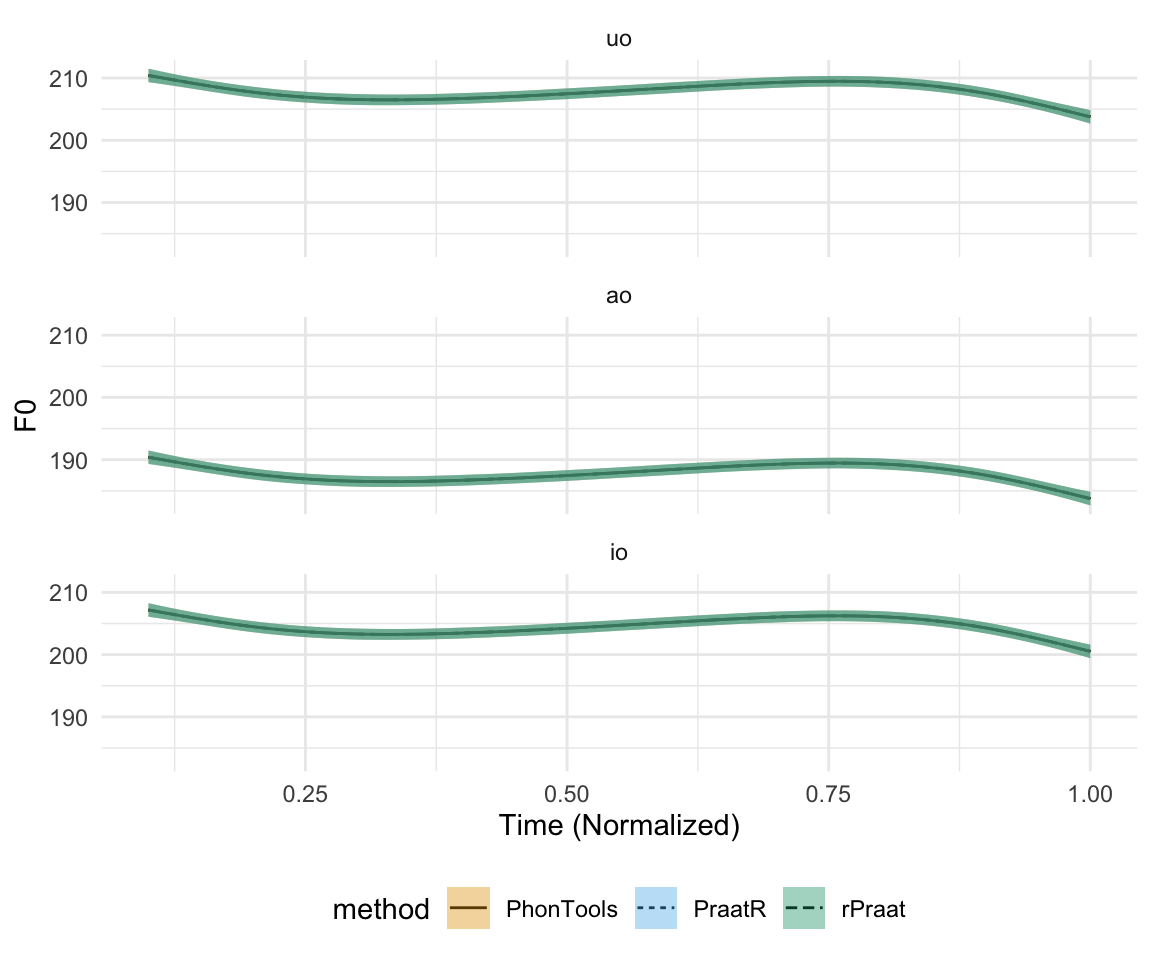
ggplot(mycomparison, aes(X, ss.Fit, group = label)) +geom_line(aes(linetype = label)) + geom_ribbon(aes(ymax = ss.upper.CI.Y, ymin = ss.lower.CI.Y, fill = label), alpha = 0.4 )+ facet_wrap(~method, ncol = 1) + theme_minimal() + scale_fill_manual(values = cbPalette[2:4]) + ylab("OP") + xlab("Time (Normalized)") + theme(legend.position="bottom")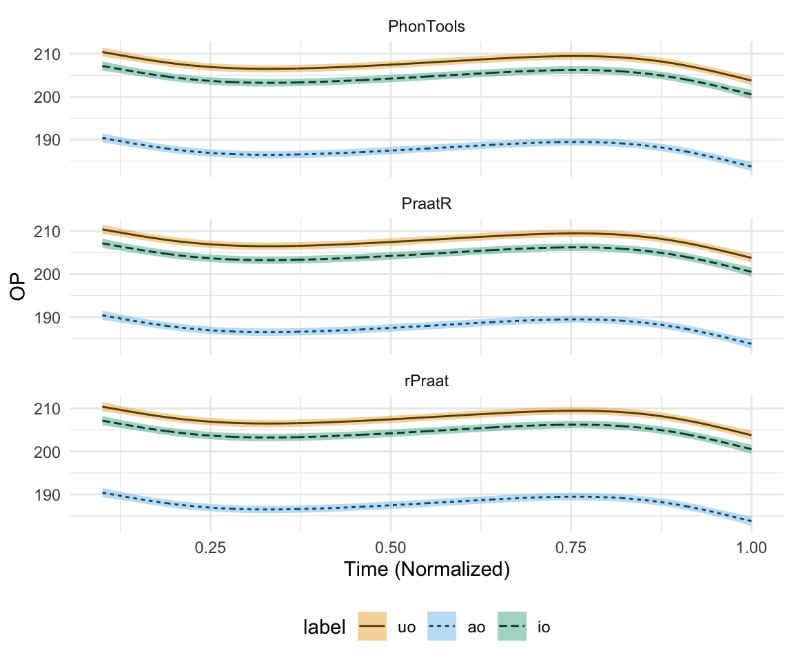
Plotting Formants - PhonR and ggplot
PhonR
PhonR allows you to plot vowel spaces, including but not limited to scatter plots, ellipses, and means.
library(linguisticsdown)
remapping <- c(ao = "ɑ", io = "i", uo = "u")
all_formant_data_PhonTools$unicodevowel <- remapping[as.character(all_formant_data_PhonTools$label)]

with(all_formant_data_PhonTools, plotVowels(f1_mdpt, f2_mdpt, label, plot.tokens = TRUE, pch.tokens = unicodevowel, cex.tokens = 1.2, alpha.tokens = 0.4, plot.means = TRUE, pch.means = unicodevowel,     cex.means = 4, var.col.by = unicodevowel, pretty = TRUE))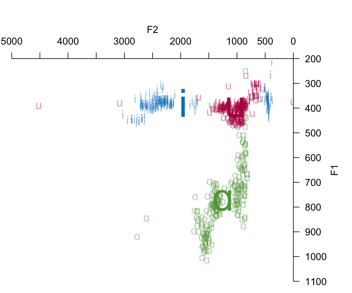
with(all_formant_data_PhonTools, plotVowels(f1_mdpt, f2_mdpt, label, plot.tokens = FALSE, plot.means = TRUE,
    var.col.by = label, var.sty.by = label, pretty = TRUE))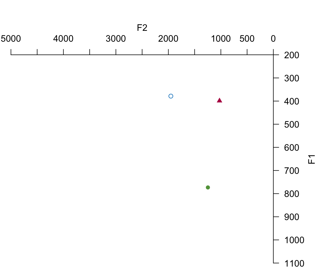
with(all_formant_data_PhonTools, plotVowels(f1_mdpt, f2_mdpt, label, plot.tokens = TRUE, pch.tokens = label, cex.tokens = 1.2, alpha.tokens = 0.2, plot.means = TRUE, pch.means = unicodevowel, cex.means = 2, var.col.by = label, ellipse.line = TRUE, pretty = TRUE))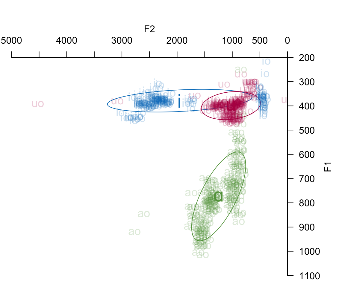
ggplot2
I personally like ggplot2 a lot more. It is extremely customizable, and can be used in any color scheme. IPA can also be used in ggplot2.
ggplot(all_formant_data_PhonTools, aes(x = f2_mdpt, y = f1_mdpt, color = label)) + geom_point(alpha = 0.4) + scale_x_reverse() + scale_y_reverse() + scale_color_manual(values = cbPalette[2:4]) + theme_minimal()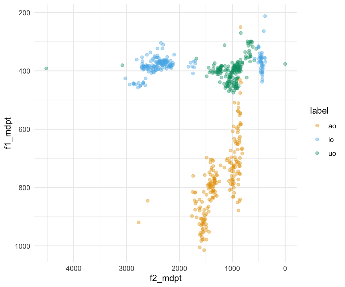
ggplot(all_formant_data_PhonTools, aes(x = f2_mdpt, y = f1_mdpt, color = label)) + geom_point(alpha = 0.4) + scale_x_reverse() + scale_y_reverse() + stat_ellipse(aes(group = label)) + scale_color_manual(values = cbPalette[2:4]) + theme_minimal()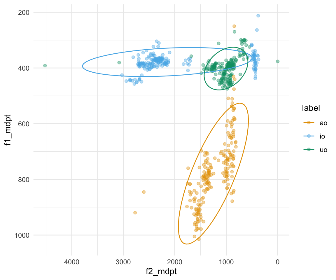
formant_means = all_formant_data_PhonTools %>% group_by(unicodevowel) %>% summarise(meanF1 = mean(f1_mdpt), meanF2 = mean(f2_mdpt))## `summarise()` ungrouping output (override with `.groups` argument)ggplot(all_formant_data_PhonTools, aes(x = f2_mdpt, y = f1_mdpt, color = unicodevowel)) + geom_point(alpha = 0.4) + scale_x_reverse() + scale_y_reverse() + stat_ellipse(aes(group = label)) +geom_text(data = formant_means, aes(x = meanF2, y = meanF1, color = unicodevowel, label = unicodevowel), size = 10) +scale_color_manual(values = cbPalette[2:4]) + theme_minimal() +
theme(legend.position='none')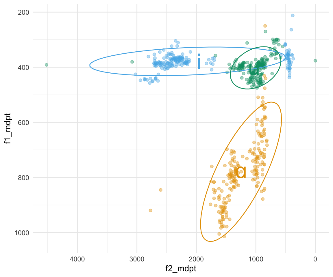
ggplot(all_formant_data_PhonTools, aes(x = f2_mdpt, y = f1_mdpt, color = unicodevowel)) + geom_point(alpha = 0.2) + scale_x_reverse() + scale_y_reverse() + stat_ellipse(aes(group = label)) +geom_text(data = formant_means, aes(x = meanF2, y = meanF1, color = unicodevowel, label = unicodevowel), size = 10) +scale_color_manual(values = cbPalette[2:4]) + theme_minimal() 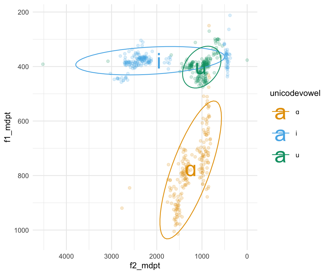
ggplot(all_formant_data_PhonTools, aes(x = f2_mdpt, y = f1_mdpt, color = unicodevowel)) + geom_point(alpha = 0.2) + scale_x_reverse(position = "top") + scale_y_reverse(position = "right") + stat_ellipse(aes(group = label)) +geom_text(data = formant_means, aes(x = meanF2, y = meanF1, color = unicodevowel, label = unicodevowel), size = 10) +scale_color_manual(values = cbPalette[2:4]) + theme_minimal() 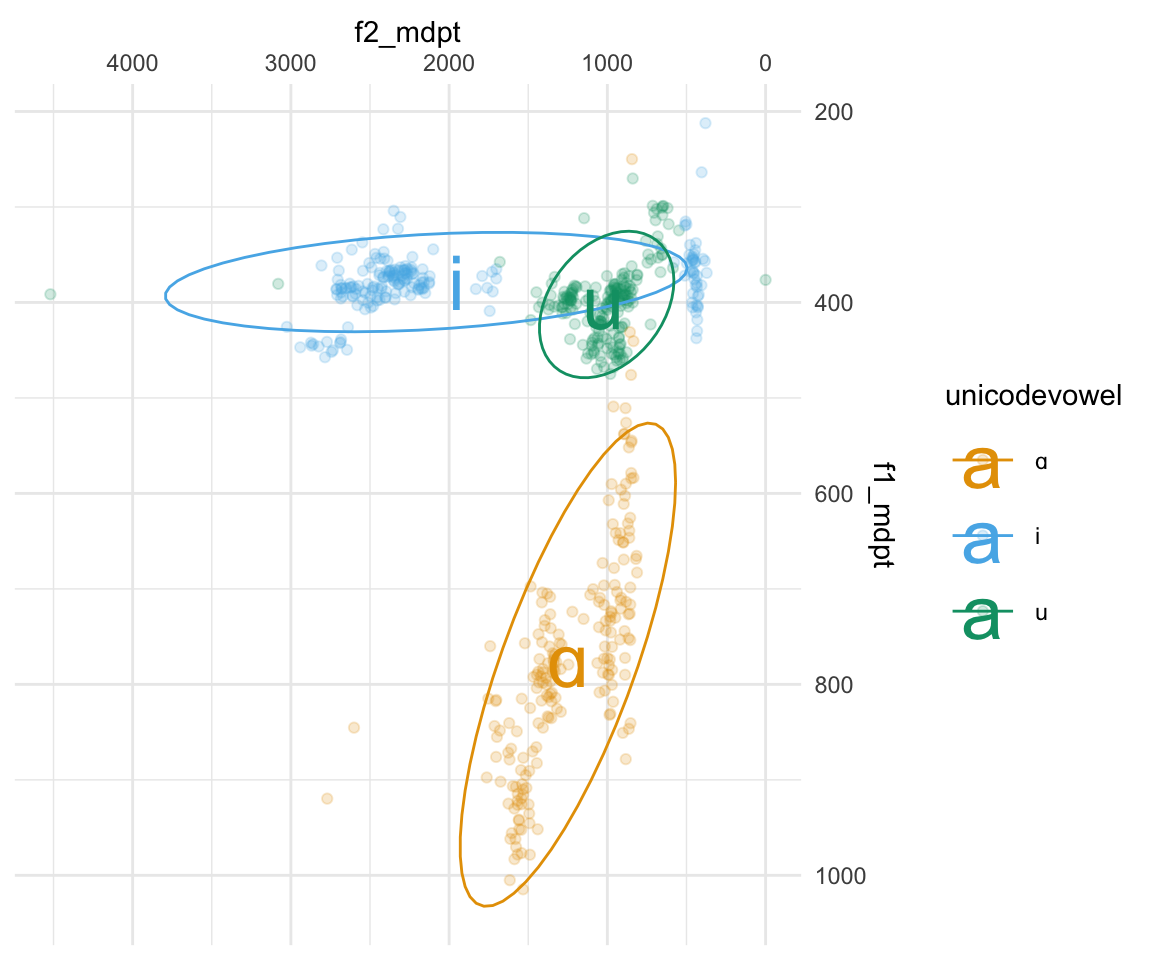
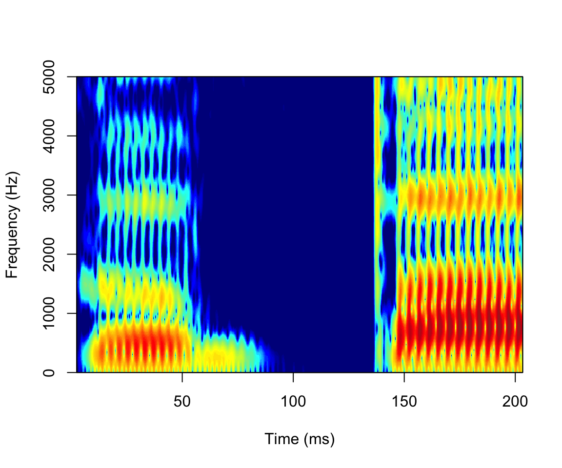
Spectrograms with PhonTools
soundmini = sound = makesound((sndWav@left / (2^(sndWav@bit-1)))[1:10000], mydir[1], fs = sndWav@samp.rate)

spectrogram(soundmini)