Ordinal logistic regression in R
Packages
The packages you will need for this workshop are as follows. I am also including the hex codes for a colorblind-friendly palette, which I use for my plots.
library(tidyverse)
library(ordinal)
library(MASS)
library(ggeffects)
library(effects)
cbPalette <- c("#999999", "#E69F00", "#56B4E9", "#009E73", "#F0E442", "#0072B2", "#D55E00", "#CC79A7")
What is ordinal logistic regression?
Ordinal logistic regression (henceforth, OLS) is used to determine the relationship between a set of predictors and an ordered factor dependent variable. This is especially useful when you have rating data, such as on a Likert scale. OLS is more appropriate to use than linear mixed effects models in this case because although a Likert scale might include numeric values to choose from, these values are inherently categorical. For example, it is unacceptable to choose 2.743 on a Likert scale ranging from 1 to 5. The most common form of an ordinal logistic regression is the “proportional odds model”.
Note that an assumption of ordinal logistic regression is the distances between two points on the scale are approximately equal. (That is, if on a scale of 1 to 5, the distance between 1 and 2 is similar to the distance between 4 and 5.) This is a difficult assumption to test, as it involves knowledge about the rating system of language users. We will therefore assume for this workshop that this is the case.
There are two packages that currently run ordinal logistic regression. The polr() function in the MASS package works, as do the clm() and clmm() functions in the ordinal package. Here, I will show you how to use the ordinal package. Note that the difference between the clm() and clmm() functions is the second m, standing for mixed. This package allows the inclusion of mixed effects. The results from the two packages are comparable.
The coefficients for OLS are given in ordered logits, or ordered log odds ratios. It is therefore important to remember what a log odds ratio is.
Probabilities, odds, and odds ratios
Recall the difference between odds and probabilities. Probabilities are considered proportions or percentages, defined by dividing the occurrences of an event divided by the total number of observations. Odds are the ratio of the probability of one event to the probability of another event, which can be simplified as the ratio of the frequency of X to the frequency of Y.
For probabilities, if the chances of two events are equal, the probability of either outcome is 0.5, or 50%. Probability ranges from 0 to 1 (0% to 100%).
If the odds equal 1, the probabilities of the outcomes are equal. If the odds are lower than 1, the probability of the second event is greater than the first (aka, if m/p < 1, then P is more likely than M). If odds is higher than 1, the probability of the first event is greater than the second event (if m/p > 1, then M more likely than P).
Log odds are logarithmically transformed odds. Log odds are also called logits. Note that logarithmically transformed here means the natural log, not base-10 log.
An odds ratio is the ratio of two odds. It tells you if the odds for a particular event is more or less likely in a particular scenario over another.
A log odds ratio is the log of the odds ratio. If a log odds ratio is positive, the specified level boosts the chances of a selected outcome. If a log odds ratio is negative, the specified level decreases the chances of a selected outcome. Log odds are centered around 0 (because ln(1) = 0, so when odds are equal, ln(odds) = 0.
In order to convert from log odds ratios to odds ratios, use exp(X). To convert from log odds ratios to probabilities, use the following formula: probability = exp(X)/(1 + exp(X)). You can also use the plogis() function to do this conversion.
| Probability | Odds | Logit |
|---|---|---|
| 0.001 | 0.001 | -6.91 |
| 0.01 | 0.01 | -4.6 |
| 0.05 | 0.05 | -2.94 |
| 0.01 | 0.11 | -2.2 |
| 0.25 | 0.33 | -1.1 |
| 0.5 | 1 | 0 |
| 0.75 | 3 | 1.1 |
| 0.9 | 9 | 2.2 |
| 0.95 | 19 | 2.94 |
| 0.99 | 99 | 4.6 |
| 0.999 | 999 | 6.91 |
Set-up of the model
The format of the OLS proportional odds model is as follows. Note that this will become important when we calculate log odds ratios, and by extension, probabilities, of events getting a certain rating (or below).
\(logit[P(Y \leq j)] = \alpha_j - \beta x, j = 1 ... J-1\)
We can read this as such: The log odds of the probability of getting a rating less than or equal to J is equal to the equation \(\alpha_j - \beta x\), where \(\alpha_j\) is the threshold coefficient corresponding to the particular rating, \(\beta\) is the variable coefficient corresponding to a change in a predictor variable, and \(x\) is the value of the predictor variable. Note, \(\beta\) is the value given to each coefficient corresponding to a variable, which is similar to a coefficient in a linear model. However, while we have in a linear model the coefficient for a variable in the original units of the response variable, this model gives us the change in log odds. The \(\alpha\) value can be considered an intercept of sorts (if comparing to a linear model) - it is the intercept for getting a rating of J or below, again in log odds.
Since we have defined the relationship between probability and log odds as P(X) = exp(X)/(1 + exp(X)) (where X is the log odds ratio), we can extend our definition of the proportional odds model to be:
\(P(Y \leq j) = \frac{exp(\alpha_j - \beta x)}{1+exp(\alpha_j - \beta x)}, j = 1 ... J-1\).
Running an ordinal logistic regression in R
Data
The data I will be using was kindly provided by Prof. Ionin. The data is comprised of ratings of acceptability of Brazilian Portuguese noun phrases in a variety of positions. The fixed effects of interest are as follows:
- NP type (bare singular vs. bare plural)
- position (subject vs. object)
- NP number (single-NP vs. list-NP)
In addition, because these are categorical variables, I have simulated a fourth fixed effect, called FreqSim, which is a numeric value between 1 and 10. While data analysis should not include the simulation of random variables, I have done this in order to show you the effect of continuous variables on a model.
##    ID   survey list     label position      NP rating  item  FreqSim
## 1 100 listNP      1 3.1barepl   object barepl       4 3.1xx 2.595569
## 2 100 listNP      1 3.2barepl   object barepl       4 3.2xx 2.507130
## 3 100 listNP      1 3.3barepl   object barepl       4 3.3xx 1.782511
## 4 100 listNP      1 3.4barepl   object barepl       4 3.4xx 1.683113
## 5 101 listNP      1 3.1barepl   object barepl       3 3.1xx 1.722588
## 6 101 listNP      1 3.2barepl   object barepl       4 3.2xx 1.396689
## 'data.frame': 1152 obs. of 9 variables:
## $ ID : int 100 100 100 100 101 101 101 101 102 102 ...
## $ survey : Factor w/ 2 levels "listNP","singleNP": 1 1 1 1 1 1 1 1 1 1 ...
## $ list : int 1 1 1 1 1 1 1 1 1 1 ...
## $ label : chr "3.1barepl" "3.2barepl" "3.3barepl" "3.4barepl" ...
## $ position: Factor w/ 2 levels "object","subject": 1 1 1 1 1 1 1 1 1 1 ...
## $ NP : Factor w/ 2 levels "barepl ","baresg": 1 1 1 1 1 1 1 1 1 1 ...
## $ rating : Ord.factor w/ 4 levels "1"<"2"<"3"<"4": 4 4 4 4 3 4 4 4 4 4 ...
## $ item : chr "3.1xx" "3.2xx" "3.3xx" "3.4xx" ...
## $ FreqSim : num 2.6 2.51 1.78 1.68 1.72 ...head(BrP)## ID survey list label position NP rating item FreqSim
## 1 100 listNP 1 3.1barepl object barepl 4 3.1xx 2.595569
## 2 100 listNP 1 3.2barepl object barepl 4 3.2xx 2.507130
## 3 100 listNP 1 3.3barepl object barepl 4 3.3xx 1.782511
## 4 100 listNP 1 3.4barepl object barepl 4 3.4xx 1.683113
## 5 101 listNP 1 3.1barepl object barepl 3 3.1xx 1.722588
## 6 101 listNP 1 3.2barepl object barepl 4 3.2xx 1.396689str(BrP)## 'data.frame': 1152 obs. of 9 variables:
## $ ID : int 100 100 100 100 101 101 101 101 102 102 ...
## $ survey : Factor w/ 2 levels "listNP","singleNP": 1 1 1 1 1 1 1 1 1 1 ...
## $ list : int 1 1 1 1 1 1 1 1 1 1 ...
## $ label : chr "3.1barepl" "3.2barepl" "3.3barepl" "3.4barepl" ...
## $ position: Factor w/ 2 levels "object","subject": 1 1 1 1 1 1 1 1 1 1 ...
## $ NP : Factor w/ 2 levels "barepl ","baresg": 1 1 1 1 1 1 1 1 1 1 ...
## $ rating : Ord.factor w/ 4 levels "1"<"2"<"3"<"4": 4 4 4 4 3 4 4 4 4 4 ...
## $ item : chr "3.1xx" "3.2xx" "3.3xx" "3.4xx" ...
## $ FreqSim : num 2.6 2.51 1.78 1.68 1.72 ...Before we get started, we should plot the data and see if we see any patterns. To do so, I will use ggplot2 syntax.
BrP %>% mutate(rating = ordered(rating, levels=rev(levels(rating)))) %>% ggplot( aes(x = position, fill = rating)) + geom_bar(position = "fill") + facet_grid(survey~NP) + scale_fill_manual(values = cbPalette) + theme_minimal()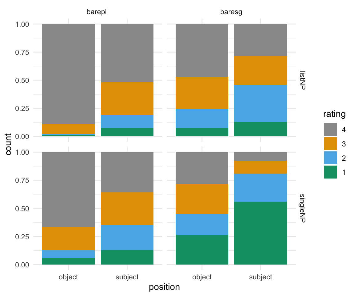
Initial model
The syntax for an OLS is similar to that of a linear mixed effects model using lme4. I will first plot the data based on the variables we are considering, and then run the model.
BrP %>% mutate(rating = ordered(rating, levels=rev(levels(rating))), position = as.factor(position)) %>% ggplot( aes(x = position, fill = rating)) + geom_bar(position = "fill") + scale_fill_manual(values = cbPalette) + theme_minimal()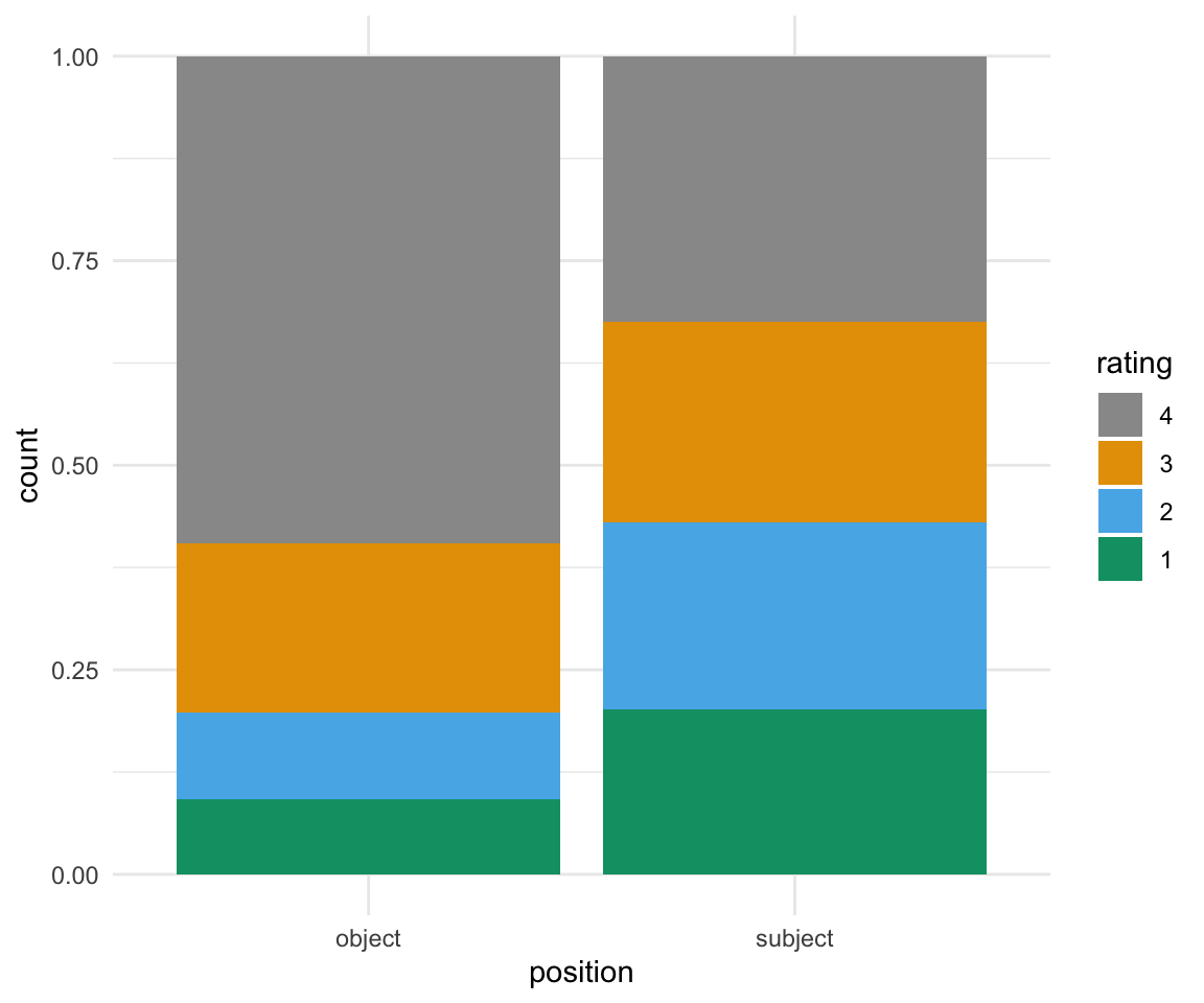
ols1 = clm(rating~position,data = BrP, link = "logit")
summary(ols1)
## formula: rating ~ position
## data: BrP
##
## link threshold nobs logLik AIC niter max.grad cond.H
## logit flexible 1152 -1419.08 2846.17 4(0) 4.77e-07 2.3e+01
##
## Coefficients:
## Estimate Std. Error z value Pr(>|z|)
## positionsubject -1.095 0.113 -9.693 <2e-16 ***
## ---
## Signif. codes: 0 '***' 0.001 '**' 0.01 '*' 0.05 '.' 0.1 ' ' 1
##
## Threshold coefficients:
## Estimate Std. Error z value
## 1|2 -2.41897 0.11131 -21.733
## 2|3 -1.39129 0.09292 -14.973
## 3|4 -0.37825 0.08329 -4.541What does this mean? We have one variable coefficient, corresponding to the difference between the two positions (similar to the slope estimate in linear models), and three threshold coefficients.
The coefficient, here just for position = subject, takes the \(\beta\) value in our model specification given above.
We can consider the coefficient similarly to coefficients in linear models. Compared to position = object, the variable position = subject has a log-odds value of -1.095. That means when we calculate the log odds ratios, whenever we are looking at an observation with position = subject, we include the \(\beta\) as -1.095, and \(x\) = 1. When we are looking at an observation with position = object, we include the \(\beta\) as -1.095, and \(x\) = 0.
In terms of its actual meaning in relationship to the variables, we would say that for a one unit increase in position (i.e., going from 0 to 1, or object to subject), we expect a -1.095 increase (or a 1.095 decrease) in the expected value of rating on the log odds scale, given all of the other variables in the model are held constant. In other words, when going from object to subject, the likelihood of a 4 versus a 1-3 on the rating scale decreases by 1.095 on the log odds scale, the likelihood of a 3 versus a 1-2 on the rating scale decreases by 1.095 on the log odds scale, and the likelihood of a 2 versus a 1 on the rating scale decreases by 1.095 on the log odds scale.
If we want to look at this on the odds scale, we can exponentiate using exp() to look at odds.
exp(coef(ols1))## 1|2 2|3 3|4 positionsubject
## 0.08901285 0.24875433 0.68505888 0.33439899Now, when position = subject, the likelihood of a 4 versus a 1-3 on the rating scale is multiplied by 0.2488 (compared to the likelihood of position = object), the likelihood of a 3 versus a 1-2 on the rating scale is multiplied by 0.2488, and the likelihood of a 2 versus a 1 on the rating scale is multiplied by 0.2488.
Now, what about the threshold coefficients? These are the coefficients, again in log odds, for receiving a rating of below J. They can be considered the “cut points” or thresholds between the two variables. So the coefficient reading 1|2 is the likelihood of receiving a 1 rating as opposed to a 2, 3, or 4 rating, the coefficient 2|3 is the likelihood of receiving a 1 or 2 as opposed to a 3 or 4, and the 3|4 coefficient is the likelihood of receiving a 1, 2, or 3, as opposed to a 4.
Why is this relevant? Because we can use the formula given above to calculate the log odds, and therefore the probability by extension, of receiving a certain score or below for each value of the predictor variable. We can also extend this to get the log odds ratio of receiving an exact rating.
First, let’s look at the log odds of receiving a 2 or below for both subject and object positions. The calculation looks like this:
Subject:
\(logit[P(Y \leq 2)] = \alpha_{2|3} - \beta (subject) = -1.39129 - (-1.095 \times 1) = -0.29629\)
Object: \(logit[P(Y \leq 2)] = \alpha_{2|3} - \beta (subject) = -1.39129 - (-1.095 \times 0) = -1.39129\)
If we want to get the probabilities for each of these, we can use the formula given above:
Subject:
\(P(Y \leq 2) = \frac{exp(\alpha_{2|3} - \beta (subject))}{1+exp(\alpha_{2|3} - \beta (subject)} = \frac{exp(-0.29629)}{1+exp(-0.29629)} = \frac{0.2487542}{1+0.2487542} = 0.4264647\)
Object: \(P(Y \leq 2) = \frac{exp(\alpha_{2|3} - \beta (subject))}{1+exp(\alpha_{2|3} - \beta (subject)} = \frac{exp(-1.39129)}{1+exp(-1.39129)} = \frac{1.097374}{2.097374} = 0.1992019\)
Note, you can also do this calculation using the plogis function:
#subject
plogis(-0.29629)
## [1] 0.4264647#object
plogis(-1.39129)## [1] 0.1992019What about the probability of getting a rating of exactly 2? We can calculate this as \(P(Y = 2) = P(Y \leq 2) - P(Y \leq 1)\).
For subject position, \(P(Y \leq 2) = 0.4264647\). Using the calculations above, we can see that \(P(Y \leq 1) = plogis(-2.41897 - (-1.095 * 1)) = 0.2101585\). Therefore, $P(Y = 2) = 0.4264647 - 0.2101585 = 0.2163062
For object position, \(P(Y \leq 2) = 0.1992019\). Using the calculations above, we can see that \(P(Y \leq 1) = plogis(-2.41897 - (-1.095 * 0)) = 0.08173753\). Therefore, $P(Y = 2) = 0.1992019 - 0.08173753 = 0.1174644
Finally, what about the probabilities/logits for the rating level 4? Since probability needs to add up to 1, we can take the probabilitiies for 1, 2, and 3, and subtract them from 1. If we would like to convert to logits, we can use the inverse of the equation above… or the qlogis() function.
Note that these results look similar to the proportions seen in the graph (though are not identical, due to the modeling parameters.)
Note that we can calculate all of these probabilties using the ggpredict() function from the ggeffects package, or using predict() in base R. I will continue using the ggpredict() version because it automatically gives confidence intervals.
newdat= data.frame(position = c("subject", "object")) %>% mutate(position = as.factor(position))
ols1predict =cbind(newdat, predict(ols1, newdat, type = "prob")$fit)
ols1predict
## position 1 2 3 4
## 1 subject 0.21022759 0.2163400 0.2454159 0.3280165
## 2 object 0.08173719 0.1174648 0.2073469 0.5934511ggpredictions_ols1 = ggpredict(ols1, terms = c("position"))
ggpredictions_ols1##
## # Predicted probabilities of rating
## # x = position
##
## # Response Level = 1
##
## x | Predicted | 95% CI
## ----------------------------------
## object | 0.08 | [0.06, 0.10]
## subject | 0.21 | [0.18, 0.25]
##
## # Response Level = 2
##
## x | Predicted | 95% CI
## ----------------------------------
## object | 0.12 | [0.10, 0.14]
## subject | 0.22 | [0.19, 0.25]
##
## # Response Level = 3
##
## x | Predicted | 95% CI
## ----------------------------------
## object | 0.21 | [0.18, 0.24]
## subject | 0.25 | [0.22, 0.28]
##
## # Response Level = 4
##
## x | Predicted | 95% CI
## ----------------------------------
## object | 0.59 | [0.55, 0.64]
## subject | 0.33 | [0.29, 0.37]#Note that ggpredicts doesn't give the original labels for position - you need to give it the names of the factor labels, which will be in the order of the original model.
ggpredictions_ols1$x = factor(ggpredictions_ols1$x)
levels(ggpredictions_ols1$x) = c("object", "subject")
colnames(ggpredictions_ols1)[c(1, 5)] = c("Position", "Rating")
ggpredictions_ols1##
## # Predicted probabilities of rating
## # x = position
##
## Position | Predicted | Rating | 95% CI
## --------------------------------------------
## object | 0.08 | 1 | [0.06, 0.10]
## object | 0.12 | 2 | [0.10, 0.14]
## object | 0.21 | 3 | [0.18, 0.24]
## object | 0.59 | 4 | [0.55, 0.64]
## subject | 0.21 | 1 | [0.18, 0.25]
## subject | 0.22 | 2 | [0.19, 0.25]
## subject | 0.25 | 3 | [0.22, 0.28]
## subject | 0.33 | 4 | [0.29, 0.37]ggplot(ggpredictions_ols1, aes(x = Rating, y = predicted)) + geom_point(aes(color = Position), position =position_dodge(width = 0.5)) + geom_errorbar(aes(ymin = conf.low, ymax = conf.high, color = Position), position = position_dodge(width = 0.5), width = 0.3) + theme_minimal() + scale_color_manual(values = cbPalette[2:3])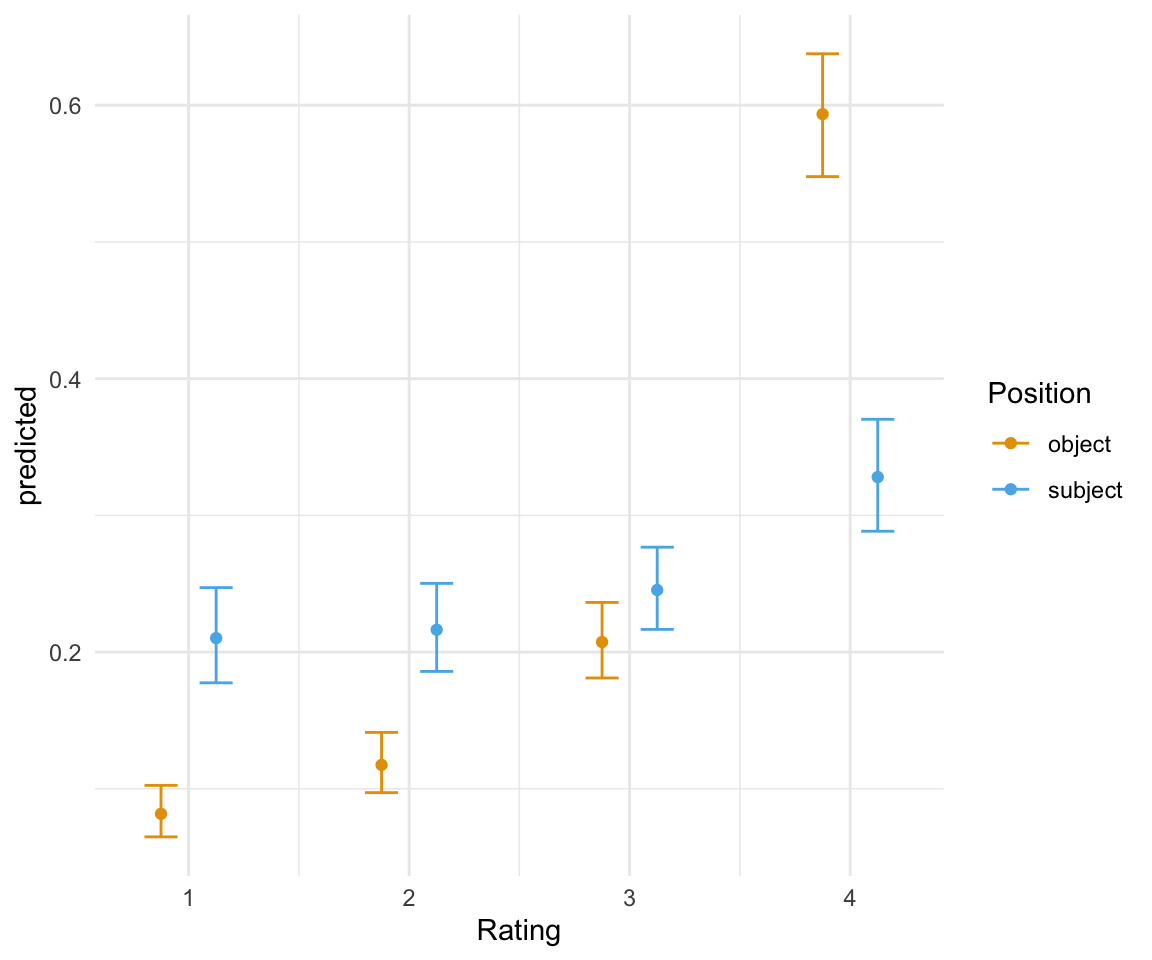
Adding another term
Now, let’s run another model, here with two terms. Can you figure out how to interpret these results?
BrP %>% mutate(rating = ordered(rating, levels=rev(levels(rating)))) %>% ggplot( aes(x = position, fill = rating)) + geom_bar(position = "fill") + scale_fill_manual(values = cbPalette) + theme_minimal()+ facet_wrap(~NP)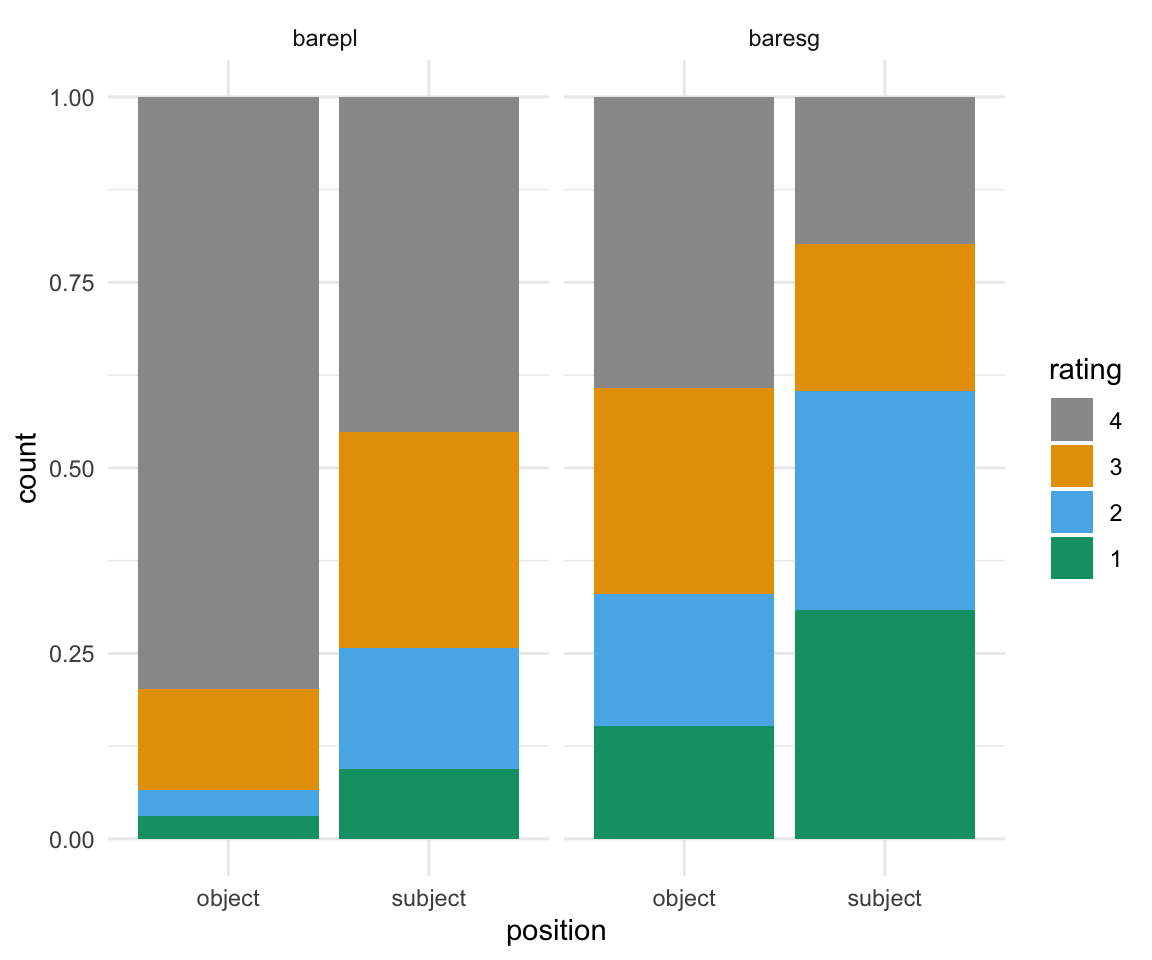
ols2 = clm(rating~position + NP,data = BrP, link = "logit")
summary(ols2)
## formula: rating ~ position + NP
## data: BrP
##
## link threshold nobs logLik AIC niter max.grad cond.H
## logit flexible 1152 -1327.81 2665.63 4(0) 6.61e-07 3.4e+01
##
## Coefficients:
## Estimate Std. Error z value Pr(>|z|)
## positionsubject -1.2492 0.1178 -10.60 <2e-16 ***
## NPbaresg -1.5581 0.1195 -13.04 <2e-16 ***
## ---
## Signif. codes: 0 '***' 0.001 '**' 0.01 '*' 0.05 '.' 0.1 ' ' 1
##
## Threshold coefficients:
## Estimate Std. Error z value
## 1|2 -3.4937 0.1487 -23.49
## 2|3 -2.3564 0.1273 -18.51
## 3|4 -1.2032 0.1115 -10.80Here, we can extend our model in a similar method we would use for a linear model:
\(logit[P(Y \leq j)] = \alpha_j - \beta_1 x_1 - \beta_2 x_2, j = 1 ... J-1\)
So what would the logit be for position = subject and NP = barepl, for a rating of 3 or less?
\(logit[P(Y \leq 3)] = \alpha_{3|4} - \beta_{subject} x_1 - \beta_{baresg} x_2 = -1.2032 - (-1.2492 \times 1) - (-1.5581 \times 0) = 0.046\)
To get probability, we use plogis():
plogis(0.046)## [1] 0.511498What about for position = object and NP = baresg, with rating == 3?
\(logit[P(Y \leq 3)] = \alpha_{3|4} - \beta_{subject} x_1 - \beta_{baresg} x_2 = -1.2032 - (-1.2492 \times 0) - (-1.5581 \times 1) = 0.3549\)
\(logit[P(Y \leq 2)] = \alpha_{2|3} - \beta_{subject} x_1 - \beta_{baresg} x_2 = -2.3564 - (-1.2492 \times 0) - (-1.5581 \times 1) = 0.3549\)
plogis(0.3549) - plogis(-0.7983)## [1] 0.277416Once again, we can use the ggpredict() function to get all probabilities:
ggpredictions_ols2 = data.frame(ggpredict(ols2, terms = c("position", "NP")))
ggpredictions_ols2
## x predicted conf.low conf.high response.level group
## 1 object 0.02949259 0.02130969 0.04068710 1 barepl
## 2 object 0.05706886 0.04364658 0.07429811 2 barepl
## 3 object 0.14433638 0.11885852 0.17419586 3 barepl
## 4 object 0.76910217 0.72180702 0.81046804 4 barepl
## 5 object 0.12613119 0.09970982 0.15832255 1 baresg
## 6 object 0.18426038 0.15364252 0.21939808 2 baresg
## 7 object 0.27739525 0.24472316 0.31262378 3 baresg
## 8 object 0.41221318 0.35853232 0.46806668 4 baresg
## 9 subject 0.09582361 0.07464488 0.12221766 1 barepl
## 10 subject 0.15257022 0.12539854 0.18438826 2 barepl
## 11 subject 0.26308316 0.23064212 0.29831791 3 barepl
## 12 subject 0.48852301 0.43302368 0.54430675 4 barepl
## 13 subject 0.33482478 0.28420004 0.38955957 1 baresg
## 14 subject 0.27602253 0.23849848 0.31699280 2 baresg
## 15 subject 0.22172775 0.19099760 0.25583859 3 baresg
## 16 subject 0.16742494 0.13554617 0.20502302 4 baresgggpredictions_ols2$x = factor(ggpredictions_ols2$x)
levels(ggpredictions_ols2$x) = c("object", "subject")
colnames(ggpredictions_ols2)[c(1, 5,6)] =c("Position", "Rating", "NP")
ggpredictions_ols2## Position predicted conf.low conf.high Rating NP
## 1 object 0.02949259 0.02130969 0.04068710 1 barepl
## 2 object 0.05706886 0.04364658 0.07429811 2 barepl
## 3 object 0.14433638 0.11885852 0.17419586 3 barepl
## 4 object 0.76910217 0.72180702 0.81046804 4 barepl
## 5 object 0.12613119 0.09970982 0.15832255 1 baresg
## 6 object 0.18426038 0.15364252 0.21939808 2 baresg
## 7 object 0.27739525 0.24472316 0.31262378 3 baresg
## 8 object 0.41221318 0.35853232 0.46806668 4 baresg
## 9 subject 0.09582361 0.07464488 0.12221766 1 barepl
## 10 subject 0.15257022 0.12539854 0.18438826 2 barepl
## 11 subject 0.26308316 0.23064212 0.29831791 3 barepl
## 12 subject 0.48852301 0.43302368 0.54430675 4 barepl
## 13 subject 0.33482478 0.28420004 0.38955957 1 baresg
## 14 subject 0.27602253 0.23849848 0.31699280 2 baresg
## 15 subject 0.22172775 0.19099760 0.25583859 3 baresg
## 16 subject 0.16742494 0.13554617 0.20502302 4 baresgggplot(ggpredictions_ols2, aes(x = Rating, y = predicted)) + geom_point(aes(color = Position), position =position_dodge(width = 0.5)) + geom_errorbar(aes(ymin = conf.low, ymax = conf.high, color = Position), position = position_dodge(width = 0.5), width = 0.3) + theme_minimal() +facet_wrap(~NP) + scale_color_manual(values = cbPalette[2:3])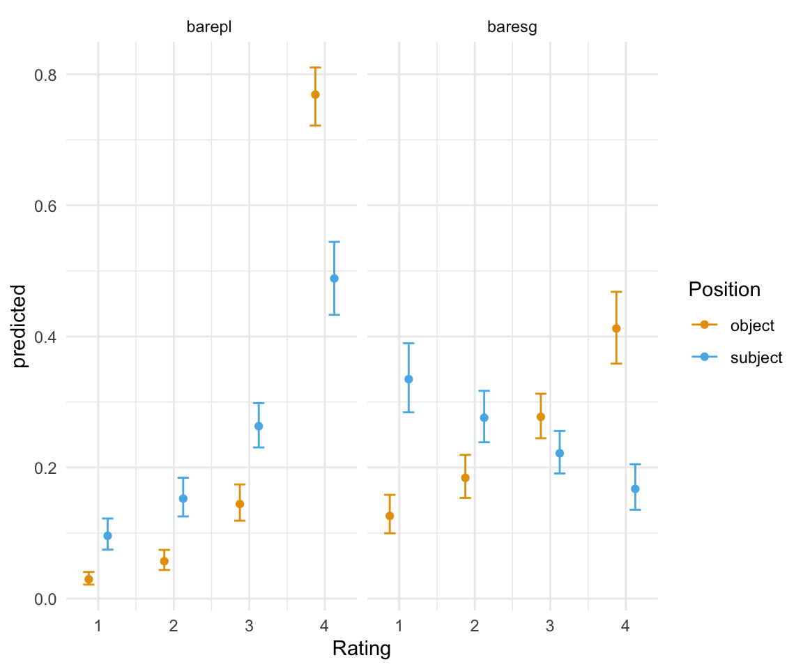
Including a continuous predictor
It is also possible to include a continuous predictor in a model. Here, I will include the FreqSim variable I simulated.
BrP %>% mutate(rating = ordered(rating, levels=rev(levels(rating)))) %>% ggplot( aes(x = FreqSim, fill = rating)) + geom_histogram(binwidth = 0.1) + scale_fill_manual(values = cbPalette) + theme_minimal() 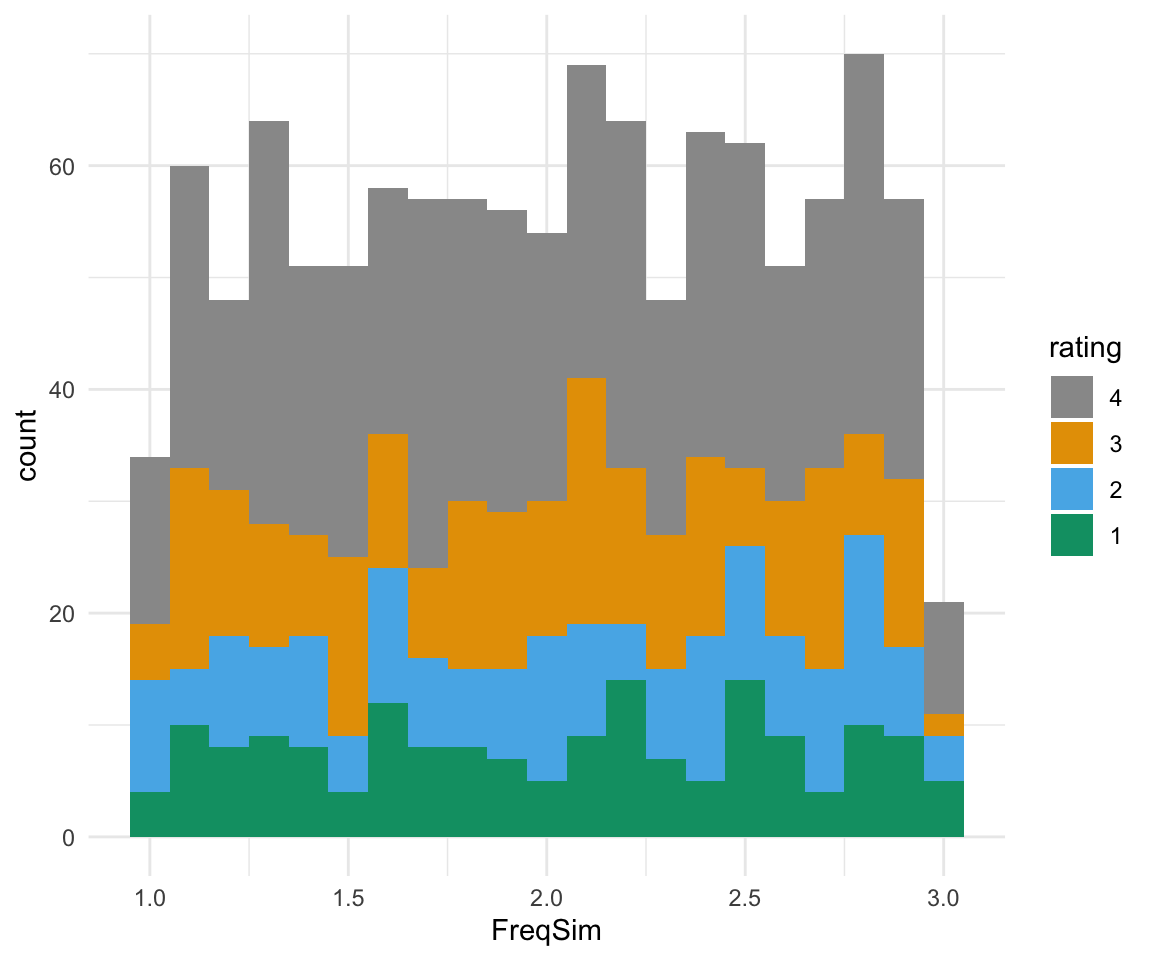
BrP %>% mutate(rating = ordered(rating, levels=rev(levels(rating)))) %>% ggplot( aes(x = cut(FreqSim, 5), fill = rating)) + geom_bar(position = "fill") + scale_fill_manual(values = cbPalette) + theme_minimal() 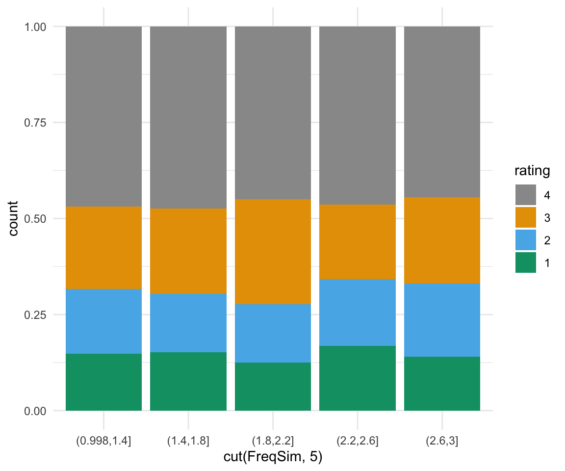
Once again you can include the continuous predictor in the model with the same syntax as for a linear model.
ols3 = clm(rating~position + FreqSim, data = BrP)
summary(ols3)
## formula: rating ~ position + FreqSim
## data: BrP
##
## link threshold nobs logLik AIC niter max.grad cond.H
## logit flexible 1152 -1419.02 2848.03 4(0) 4.77e-07 2.3e+02
##
## Coefficients:
## Estimate Std. Error z value Pr(>|z|)
## positionsubject -1.09443 0.11304 -9.682 <2e-16 ***
## FreqSim -0.03531 0.09566 -0.369 0.712
## ---
## Signif. codes: 0 '***' 0.001 '**' 0.01 '*' 0.05 '.' 0.1 ' ' 1
##
## Threshold coefficients:
## Estimate Std. Error z value
## 1|2 -2.4896 0.2215 -11.240
## 2|3 -1.4617 0.2123 -6.884
## 3|4 -0.4485 0.2078 -2.158Here, our result for FreqSim is not significant, which is not surprising since this is simulated data. However, we can still use this to show the how to interpret the results of the model. In this case, we say that for a one unit increase in FreqSim, we expect a -0.03531 increase (or a 0.03531 decrease) in the expected value of rating on the log odds scale, given all of the other variables in the model are held constant. In other words, the likelihood of a 4 versus a 1-3 on the rating scale decreases by 0.03531 on the log odds scale, the likelihood of a 3 versus a 1-2 on the rating scale decreases by 0.03531 on the log odds scale, and the likelihood of a 2 versus a 1 on the rating scale decreases by 0.03531 on the log odds scale.
If we wanted to calculate the probability of getting a rating value of 1 for a word with FreqSim = 2 and position = subject, we use our formula:
\(logit[P(Y \leq 1)] = \alpha_{1|2} - \beta_{subject} x_1 - \beta_{FreqSim} x_2 = -2.4896 - (-1.09443 \times 1) - (-0.03531 \times 3) = -1.28924\)
plogis(-1.28924)## [1] 0.2159815Once again, the ggpredict() function can be used to predict values for all combinations of the predictor variable.
ggpredictions_ols3 = data.frame(ggpredict(ols3, terms = c("position", "FreqSim [1, 1.5, 2, 2.5, 3]")))
ggpredictions_ols3
## x predicted conf.low conf.high response.level group
## 1 object 0.07912849 0.05822380 0.1066885 1 1
## 2 object 0.11453662 0.08946980 0.1455041 2 1
## 3 object 0.20448986 0.17380786 0.2390212 3 1
## 4 object 0.60184503 0.53256920 0.6672683 4 1
## 5 object 0.08042470 0.06248520 0.1029490 1 1.5
## 6 object 0.11601261 0.09451516 0.1416348 2 1.5
## 7 object 0.20595625 0.17860685 0.2362888 3 1.5
## 8 object 0.59760644 0.54519364 0.6478802 4 1.5
## 9 object 0.08174025 0.06486185 0.1025292 1 2
## 10 object 0.11749914 0.09724485 0.1413117 2 2
## 11 object 0.20740739 0.18112912 0.2363975 3 2
## 12 object 0.59335322 0.54763988 0.6375048 4 2
## 13 object 0.08307538 0.06460484 0.1062269 1 2.5
## 14 object 0.11899600 0.09696862 0.1452224 2 2.5
## 15 object 0.20884266 0.18119998 0.2394690 3 2.5
## 16 object 0.58908596 0.53589732 0.6402707 4 2.5
## 17 object 0.08443031 0.06224939 0.1135577 1 3
## 18 object 0.12050302 0.09432392 0.1527228 2 3
## 19 object 0.21026142 0.17931894 0.2449496 3 3
## 20 object 0.58480525 0.51415248 0.6521350 4 3
## 21 subject 0.20426926 0.15921706 0.2581553 1 1
## 22 subject 0.21349866 0.17933561 0.2521700 2 1
## 23 subject 0.24625350 0.21706275 0.2779761 3 1
## 24 subject 0.33597858 0.27531230 0.4025866 4 1
## 25 subject 0.20715426 0.17072961 0.2490165 1 1.5
## 26 subject 0.21491462 0.18353715 0.2500137 2 1.5
## 27 subject 0.24588026 0.21692545 0.2773312 3 1.5
## 28 subject 0.33205086 0.28588557 0.3816865 4 1.5
## 29 subject 0.21006924 0.17737136 0.2469851 1 2
## 30 subject 0.21631244 0.18584104 0.2502444 2 2
## 31 subject 0.24547195 0.21664845 0.2767753 3 2
## 32 subject 0.32814637 0.28850006 0.3704046 4 2
## 33 subject 0.21301423 0.17658792 0.2546309 1 2.5
## 34 subject 0.21769149 0.18619078 0.2528657 2 2.5
## 35 subject 0.24502879 0.21613852 0.2764189 3 2.5
## 36 subject 0.32426550 0.27944156 0.3725619 4 2.5
## 37 subject 0.21598921 0.17011998 0.2701993 1 3
## 38 subject 0.21905113 0.18492454 0.2574860 2 3
## 39 subject 0.24455102 0.21529237 0.2763855 3 3
## 40 subject 0.32040864 0.26247998 0.3844575 4 3ggpredictions_ols3$x = factor(ggpredictions_ols3$x)
levels(ggpredictions_ols3$x) = c("object", "subject")
colnames(ggpredictions_ols3)[c(1, 5,6)] =c("Position", "Rating", "FreqSim")
ggpredictions_ols3$Rating = as.factor(ggpredictions_ols3$Rating)
ggplot(ggpredictions_ols3, aes(x = FreqSim, y = predicted)) + geom_smooth(aes(color = Rating, group = Rating), se = FALSE)+ theme_minimal() +facet_wrap(~Position) + scale_color_manual(values = cbPalette)## `geom_smooth()` using method = 'loess' and formula 'y ~ x'## Warning in simpleLoess(y, x, w, span, degree = degree, parametric =
## parametric, : span too small. fewer data values than degrees of freedom.## Warning in simpleLoess(y, x, w, span, degree = degree, parametric =
## parametric, : pseudoinverse used at 0.98## Warning in simpleLoess(y, x, w, span, degree = degree, parametric =
## parametric, : neighborhood radius 2.02## Warning in simpleLoess(y, x, w, span, degree = degree, parametric =
## parametric, : reciprocal condition number 0## Warning in simpleLoess(y, x, w, span, degree = degree, parametric =
## parametric, : There are other near singularities as well. 4.0804## Warning in simpleLoess(y, x, w, span, degree = degree, parametric =
## parametric, : span too small. fewer data values than degrees of freedom.## Warning in simpleLoess(y, x, w, span, degree = degree, parametric =
## parametric, : pseudoinverse used at 0.98## Warning in simpleLoess(y, x, w, span, degree = degree, parametric =
## parametric, : neighborhood radius 2.02## Warning in simpleLoess(y, x, w, span, degree = degree, parametric =
## parametric, : reciprocal condition number 0## Warning in simpleLoess(y, x, w, span, degree = degree, parametric =
## parametric, : There are other near singularities as well. 4.0804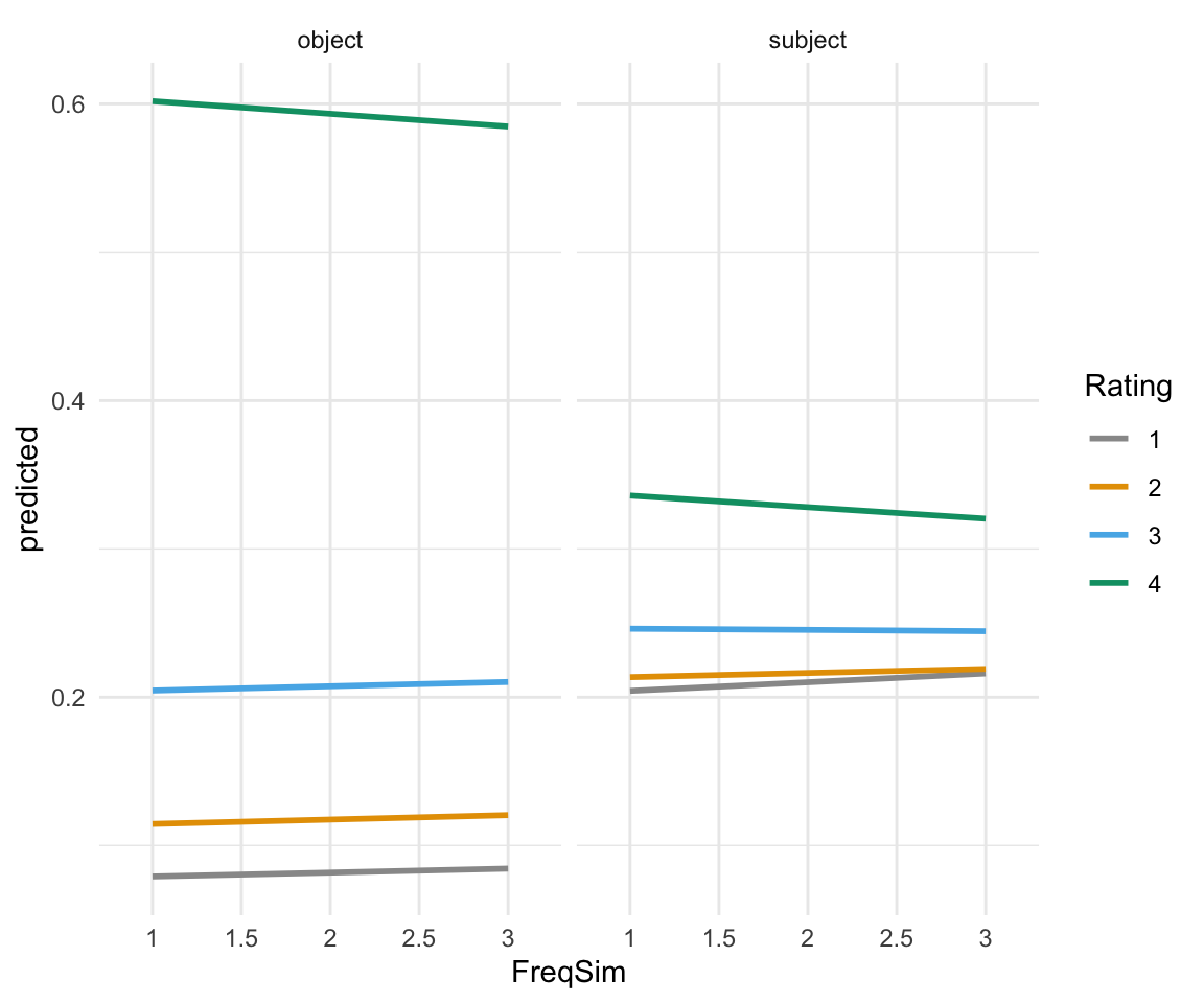
As we can see here, FreqSim really doesn’t add much. This isn’t totally surprising. A dataset with a meaningful research question behind it will possibly show more significant results.
Interactions
Including an interaction, like with a linear model, will require a theoretical motivation. I will include here a two-way interaction in order to show how the model can be interpreted with an interaction. The syntax is the same as with a linear model.
ols4 = clm(rating~position * NP,data = BrP, link = "logit")
summary(ols4)
## formula: rating ~ position * NP
## data: BrP
##
## link threshold nobs logLik AIC niter max.grad cond.H
## logit flexible 1152 -1325.63 2663.27 4(0) 3.91e-07 8.9e+01
##
## Coefficients:
## Estimate Std. Error z value Pr(>|z|)
## positionsubject -1.5325 0.1826 -8.392 <2e-16 ***
## NPbaresg -1.8399 0.1833 -10.038 <2e-16 ***
## positionsubject:NPbaresg 0.4917 0.2367 2.077 0.0378 *
## ---
## Signif. codes: 0 '***' 0.001 '**' 0.01 '*' 0.05 '.' 0.1 ' ' 1
##
## Threshold coefficients:
## Estimate Std. Error z value
## 1|2 -3.6605 0.1725 -21.218
## 2|3 -2.5350 0.1580 -16.049
## 3|4 -1.3834 0.1461 -9.469Now, we have an extra term in our model coefficients, being the interaction term. This term is significant, indicating that there is a modulating effect between the position and NP terms.
Now, our model looks like this:
\(logit[P(Y \leq j)] = \alpha_j - \beta_1 x_1 - \beta_2 x_2 - \beta_3 x_1x_2, j = 1 ... J-1\)
I will do the calculation for a rating of exactly 2, for a subject/baresg word:
\(logit[P(Y \leq 2)] = \alpha_{2|3} - \beta_{subject} x_1 - \beta_{baresg} x_2 - \beta_{subject:baresg} x_1x_2 = -2.5350 - (-1.5325 \times 1) - (-1.8399 \times 1) - (0.4917 \times 1 \times 1) = 0.3457\)
\(logit[P(Y \leq 1)] = \alpha_{1|2} - \beta_{subject} x_1 - \beta_{baresg} x_2 - \beta_{subject:baresg} x_1x_2 = -3.6605 - (-1.5325 \times 1) - (-1.8399 \times 1) - (0.4917 \times 1 \times 1) = 0.3457\)
plogis(0.3457)## [1] 0.5855745plogis(-0.7798)## [1] 0.314363plogis(0.3457) - plogis(-0.7798)## [1] 0.2712115Once again, we can plot the results:
ggpredictions_ols4 = data.frame(ggpredict(ols4, terms = c("position", "NP")))
ggpredictions_ols4
## x predicted conf.low conf.high response.level group
## 1 object 0.02507574 0.01717219 0.03648189 1 barepl
## 2 object 0.04836596 0.03455575 0.06731063 2 barepl
## 3 object 0.12702267 0.09819175 0.16279077 3 barepl
## 4 object 0.79953562 0.74191333 0.84694677 4 barepl
## 5 object 0.13936432 0.10809666 0.17787264 1 baresg
## 6 object 0.19353390 0.16103018 0.23079362 2 baresg
## 7 object 0.27928169 0.24672221 0.31434492 3 baresg
## 8 object 0.38782009 0.33007465 0.44889857 4 baresg
## 9 subject 0.10640447 0.08125202 0.13817215 1 barepl
## 10 subject 0.16203947 0.13256674 0.19657975 2 barepl
## 11 subject 0.26875191 0.23601925 0.30421648 3 barepl
## 12 subject 0.46280415 0.40195917 0.52477742 4 barepl
## 13 subject 0.31434659 0.26162291 0.37233754 1 baresg
## 14 subject 0.27120307 0.23388011 0.31205606 2 baresg
## 15 subject 0.23160509 0.19919887 0.26752207 3 baresg
## 16 subject 0.18284525 0.14560262 0.22708207 4 baresgggpredictions_ols4$x = factor(ggpredictions_ols4$x)
levels(ggpredictions_ols4$x) = c("object", "subject")
colnames(ggpredictions_ols4)[c(1, 5,6)] =c("Position", "Rating", "NP")
ggpredictions_ols4## Position predicted conf.low conf.high Rating NP
## 1 object 0.02507574 0.01717219 0.03648189 1 barepl
## 2 object 0.04836596 0.03455575 0.06731063 2 barepl
## 3 object 0.12702267 0.09819175 0.16279077 3 barepl
## 4 object 0.79953562 0.74191333 0.84694677 4 barepl
## 5 object 0.13936432 0.10809666 0.17787264 1 baresg
## 6 object 0.19353390 0.16103018 0.23079362 2 baresg
## 7 object 0.27928169 0.24672221 0.31434492 3 baresg
## 8 object 0.38782009 0.33007465 0.44889857 4 baresg
## 9 subject 0.10640447 0.08125202 0.13817215 1 barepl
## 10 subject 0.16203947 0.13256674 0.19657975 2 barepl
## 11 subject 0.26875191 0.23601925 0.30421648 3 barepl
## 12 subject 0.46280415 0.40195917 0.52477742 4 barepl
## 13 subject 0.31434659 0.26162291 0.37233754 1 baresg
## 14 subject 0.27120307 0.23388011 0.31205606 2 baresg
## 15 subject 0.23160509 0.19919887 0.26752207 3 baresg
## 16 subject 0.18284525 0.14560262 0.22708207 4 baresgggplot(ggpredictions_ols4, aes(x = Rating, y = predicted)) + geom_point(aes(color = Position), position =position_dodge(width = 0.5)) + geom_errorbar(aes(ymin = conf.low, ymax = conf.high, color = Position), position = position_dodge(width = 0.5), width = 0.3) + theme_minimal() +facet_wrap(~NP) + scale_color_manual(values = cbPalette[2:3])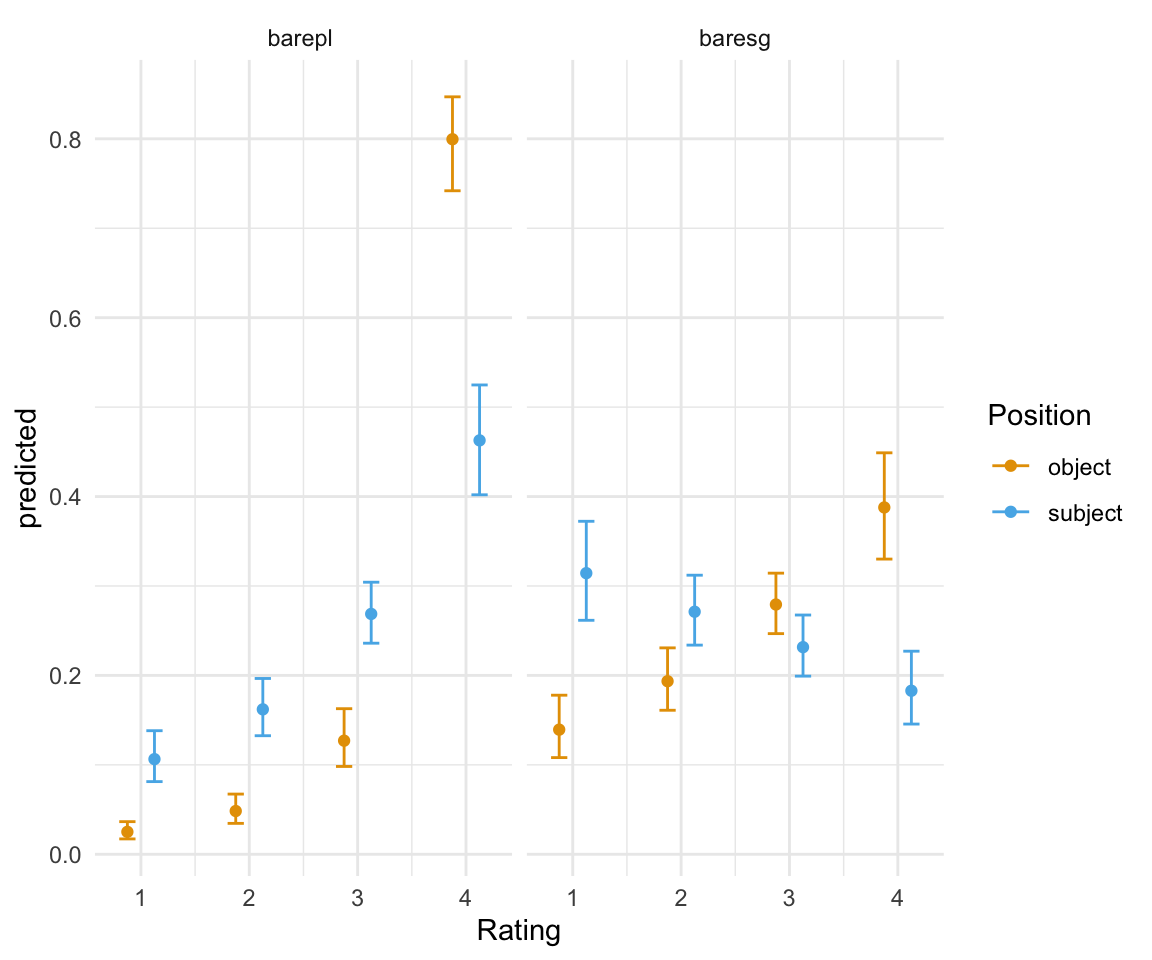
Random effects
As I mentioned before, the ordinal package has an advantage over MASS, in that it has the ability to include random effects. The syntax is similar to that of lme4’s lmer() function. Note that the function being used here is clmm() - the extra m stands for mixed.
ols5 = clmm(rating~position*NP + (1|ID), data = BrP)
summary(ols5)
## Cumulative Link Mixed Model fitted with the Laplace approximation
##
## formula: rating ~ position * NP + (1 | ID)
## data: BrP
##
## link threshold nobs logLik AIC niter max.grad cond.H
## logit flexible 1152 -1243.45 2500.90 442(1697) 1.50e-03 8.6e+01
##
## Random effects:
## Groups Name Variance Std.Dev.
## ID (Intercept) 1.265 1.125
## Number of groups: ID 72
##
## Coefficients:
## Estimate Std. Error z value Pr(>|z|)
## positionsubject -1.8757 0.1996 -9.397 <2e-16 ***
## NPbaresg -2.2848 0.2022 -11.300 <2e-16 ***
## positionsubject:NPbaresg 0.6422 0.2510 2.559 0.0105 *
## ---
## Signif. codes: 0 '***' 0.001 '**' 0.01 '*' 0.05 '.' 0.1 ' ' 1
##
## Threshold coefficients:
## Estimate Std. Error z value
## 1|2 -4.4650 0.2457 -18.170
## 2|3 -3.0915 0.2258 -13.694
## 3|4 -1.6945 0.2097 -8.081Now we have the same information as before, plus a little more. At the top of the summary, there is the information regarding the random effects - specifically the ID of the participant. The coefficients have changed slightly , though we have the same significance levels.
Note that we have an extra column in our prediction matrix, with the standard error.
ggpredictions_ols5 = data.frame(ggpredict(ols5, terms = c("position", "NP"), type = "fe"))## Loading required namespace: emmeansggpredictions_ols5## x predicted std.error conf.low conf.high response.level group
## 1 object 0.01137409 0.002763256 0.005958204 0.01678997 1 barepl
## 2 object 0.03208654 0.006904418 0.018554125 0.04561894 2 barepl
## 3 object 0.11172434 0.019023724 0.074438530 0.14901016 3 barepl
## 4 object 0.84481504 0.027491683 0.790932327 0.89869775 4 barepl
## 5 object 0.10154649 0.017748501 0.066760071 0.13633292 1 baresg
## 6 object 0.20705908 0.024420592 0.159195599 0.25492256 2 baresg
## 7 object 0.33483305 0.018034067 0.299486926 0.37017917 3 baresg
## 8 object 0.35656138 0.041163010 0.275883361 0.43723940 4 baresg
## 9 subject 0.06983095 0.012987834 0.044375260 0.09528663 1 barepl
## 10 subject 0.15884947 0.021620967 0.116473149 0.20122578 2 barepl
## 11 subject 0.31649341 0.020664737 0.275991269 0.35699555 3 barepl
## 12 subject 0.45482618 0.044261182 0.368075856 0.54157650 4 barepl
## 13 subject 0.27956441 0.036329195 0.208360493 0.35076832 1 baresg
## 14 subject 0.32556600 0.021210648 0.283993896 0.36713811 2 baresg
## 15 subject 0.25589766 0.024266581 0.208336037 0.30345929 3 baresg
## 16 subject 0.13897193 0.022345994 0.095174586 0.18276927 4 baresgggpredictions_ols5$x = factor(ggpredictions_ols5$x)
levels(ggpredictions_ols5$x) = c("object", "subject")
colnames(ggpredictions_ols5)[c(1, 6,7)] =c("Position", "Rating", "NP")
ggpredictions_ols5## Position predicted std.error conf.low conf.high Rating NP
## 1 object 0.01137409 0.002763256 0.005958204 0.01678997 1 barepl
## 2 object 0.03208654 0.006904418 0.018554125 0.04561894 2 barepl
## 3 object 0.11172434 0.019023724 0.074438530 0.14901016 3 barepl
## 4 object 0.84481504 0.027491683 0.790932327 0.89869775 4 barepl
## 5 object 0.10154649 0.017748501 0.066760071 0.13633292 1 baresg
## 6 object 0.20705908 0.024420592 0.159195599 0.25492256 2 baresg
## 7 object 0.33483305 0.018034067 0.299486926 0.37017917 3 baresg
## 8 object 0.35656138 0.041163010 0.275883361 0.43723940 4 baresg
## 9 subject 0.06983095 0.012987834 0.044375260 0.09528663 1 barepl
## 10 subject 0.15884947 0.021620967 0.116473149 0.20122578 2 barepl
## 11 subject 0.31649341 0.020664737 0.275991269 0.35699555 3 barepl
## 12 subject 0.45482618 0.044261182 0.368075856 0.54157650 4 barepl
## 13 subject 0.27956441 0.036329195 0.208360493 0.35076832 1 baresg
## 14 subject 0.32556600 0.021210648 0.283993896 0.36713811 2 baresg
## 15 subject 0.25589766 0.024266581 0.208336037 0.30345929 3 baresg
## 16 subject 0.13897193 0.022345994 0.095174586 0.18276927 4 baresgggplot(ggpredictions_ols5, aes(x = Rating, y = predicted)) + geom_point(aes(color = Position), position =position_dodge(width = 0.5)) + geom_errorbar(aes(ymin = conf.low, ymax = conf.high, color = Position), position = position_dodge(width = 0.5), width = 0.3) + theme_minimal() +facet_wrap(~NP) + scale_color_manual(values = cbPalette[2:3])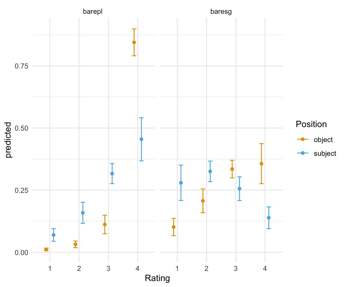
The full model
Following Dr. Ionin’s paper from which this data comes, let’s take a look at a full model. Note that this took me about 15 seconds to run on my computer.
#raw data
BrP %>% mutate(rating = ordered(rating, levels=rev(levels(rating)))) %>% ggplot( aes(x = position, fill = rating)) + geom_bar(position = "fill") + facet_grid(survey~NP) + scale_fill_manual(values = cbPalette) + theme_minimal() + ggtitle("Raw Data")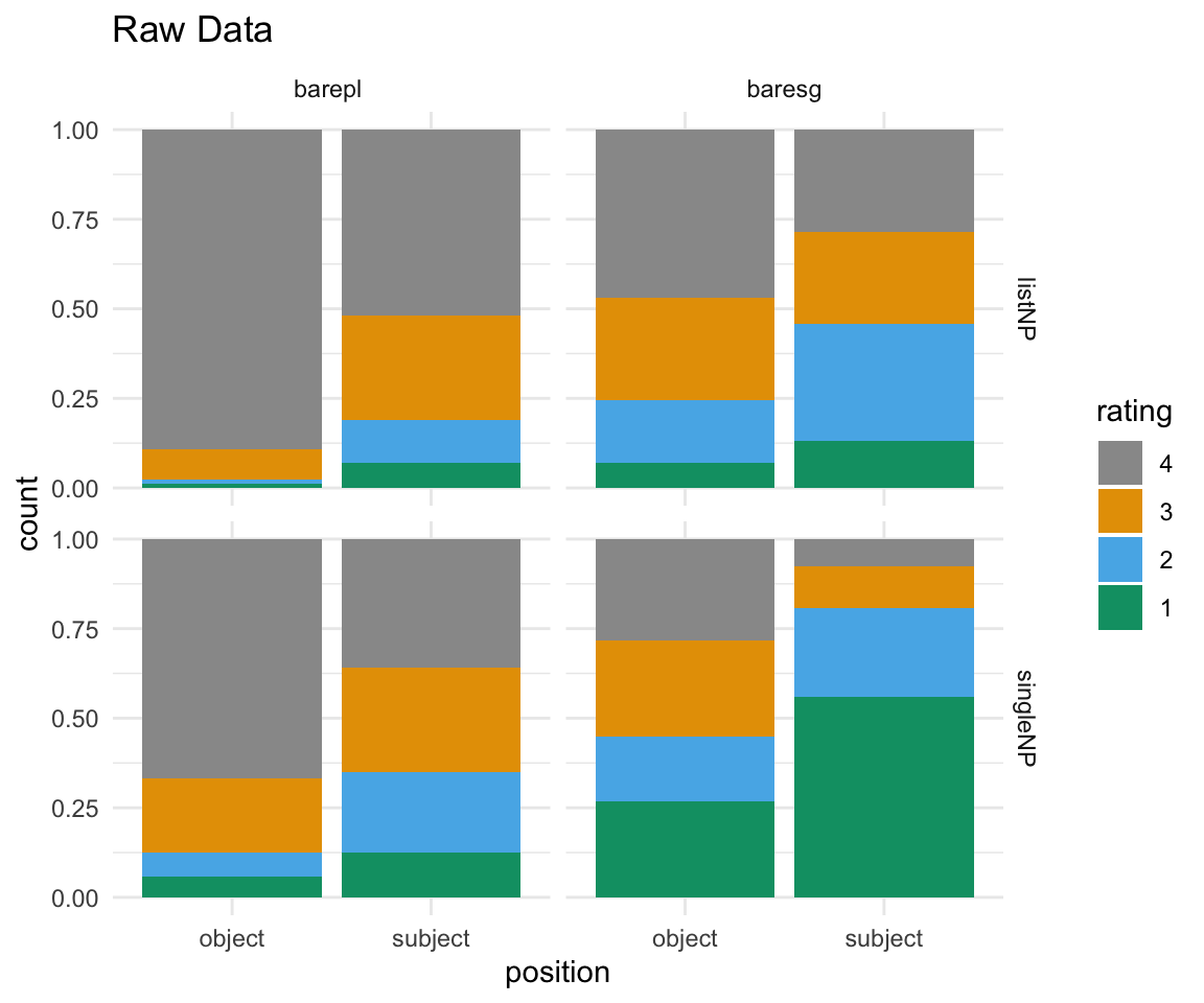
ols6 = clmm(rating~position*NP*survey + (1|ID) + (1|item), data = BrP)

summary(ols6)
## Cumulative Link Mixed Model fitted with the Laplace approximation
##
## formula: rating ~ position * NP * survey + (1 | ID) + (1 | item)
## data: BrP
##
## link threshold nobs logLik AIC niter max.grad cond.H
## logit flexible 1152 -1181.20 2386.40 979(3593) 4.39e-04 3.6e+02
##
## Random effects:
## Groups Name Variance Std.Dev.
## ID (Intercept) 1.0032 1.0016
## item (Intercept) 0.5767 0.7594
## Number of groups: ID 72, item 24
##
## Coefficients:
## Estimate Std. Error z value Pr(>|z|)
## positionsubject -2.6630 0.4504 -5.912 3.38e-09
## NPbaresg -2.9280 0.3255 -8.996 < 2e-16
## surveysingleNP -1.9855 0.4270 -4.650 3.32e-06
## positionsubject:NPbaresg 1.6000 0.3812 4.197 2.70e-05
## positionsubject:surveysingleNP 1.0033 0.4183 2.399 0.016462
## NPbaresg:surveysingleNP 0.6596 0.4172 1.581 0.113873
## positionsubject:NPbaresg:surveysingleNP -1.8573 0.5332 -3.483 0.000495
##
## positionsubject ***
## NPbaresg ***
## surveysingleNP ***
## positionsubject:NPbaresg ***
## positionsubject:surveysingleNP *
## NPbaresg:surveysingleNP
## positionsubject:NPbaresg:surveysingleNP ***
## ---
## Signif. codes: 0 '***' 0.001 '**' 0.01 '*' 0.05 '.' 0.1 ' ' 1
##
## Threshold coefficients:
## Estimate Std. Error z value
## 1|2 -5.9204 0.4285 -13.815
## 2|3 -4.3697 0.4105 -10.645
## 3|4 -2.8239 0.3945 -7.158ggpredictions_ols6 = data.frame(ggpredict(ols6, terms = c("position", "NP", "survey"), type = "fe"))
ggpredictions_ols6## x predicted std.error conf.low conf.high response.level
## 1 object 0.002676824 0.001144066 0.0004344957 0.004919153 1
## 2 object 0.009819713 0.003966276 0.0020459550 0.017593472 2
## 3 object 0.043548519 0.015966933 0.0122539060 0.074843133 3
## 4 object 0.943954943 0.020871473 0.9030476070 0.984862279 4
## 5 object 0.019172061 0.007138515 0.0051808296 0.033163293 1
## 6 object 0.065211294 0.021399504 0.0232690372 0.107153552 2
## 7 object 0.217483944 0.048145526 0.1231204464 0.311847442 3
## 8 object 0.698132700 0.074938724 0.5512554992 0.845009901 4
## 9 object 0.047769286 0.014953506 0.0184609530 0.077077618 1
## 10 object 0.143511540 0.034894762 0.0751190622 0.211904018 2
## 11 object 0.334719905 0.033750949 0.2685692596 0.400870550 3
## 12 object 0.473999270 0.077505563 0.3220911576 0.625907382 4
## 13 object 0.158884489 0.045998360 0.0687293595 0.249039618 1
## 14 object 0.312188810 0.042784764 0.2283322140 0.396045405 2
## 15 object 0.335823305 0.035862221 0.2655346435 0.406111966 3
## 16 object 0.193103397 0.053080916 0.0890667138 0.297140080 4
## 17 subject 0.037061496 0.011898905 0.0137400702 0.060382921 1
## 18 subject 0.116531310 0.030321648 0.0571019717 0.175960647 2
## 19 subject 0.306271318 0.039653973 0.2285509581 0.383991677 3
## 20 subject 0.540135877 0.077606340 0.3880302456 0.692241509 4
## 21 subject 0.093196213 0.029333044 0.0357045026 0.150687924 1
## 22 subject 0.233205815 0.047014085 0.1410599022 0.325351729 2
## 23 subject 0.368110683 0.019593769 0.3297076023 0.406513764 3
## 24 subject 0.305487288 0.071595621 0.1651624504 0.445812126 4
## 25 subject 0.126822969 0.034951905 0.0583184949 0.195327443 1
## 26 subject 0.279634215 0.042680589 0.1959817979 0.363286631 2
## 27 subject 0.356176848 0.025948068 0.3053195688 0.407034127 3
## 28 subject 0.237365968 0.056150724 0.1273125719 0.347419365 4
## 29 subject 0.562301081 0.084786699 0.3961222049 0.728479958 1
## 30 subject 0.295996488 0.045751098 0.2063259838 0.385666992 2
## 31 subject 0.107709792 0.031408243 0.0461507667 0.169268818 3
## 32 subject 0.033992639 0.011888492 0.0106916222 0.057293655 4
## group facet
## 1 barepl listNP
## 2 barepl listNP
## 3 barepl listNP
## 4 barepl listNP
## 5 barepl singleNP
## 6 barepl singleNP
## 7 barepl singleNP
## 8 barepl singleNP
## 9 baresg listNP
## 10 baresg listNP
## 11 baresg listNP
## 12 baresg listNP
## 13 baresg singleNP
## 14 baresg singleNP
## 15 baresg singleNP
## 16 baresg singleNP
## 17 barepl listNP
## 18 barepl listNP
## 19 barepl listNP
## 20 barepl listNP
## 21 barepl singleNP
## 22 barepl singleNP
## 23 barepl singleNP
## 24 barepl singleNP
## 25 baresg listNP
## 26 baresg listNP
## 27 baresg listNP
## 28 baresg listNP
## 29 baresg singleNP
## 30 baresg singleNP
## 31 baresg singleNP
## 32 baresg singleNPggpredictions_ols6$x = factor(ggpredictions_ols6$x)
levels(ggpredictions_ols6$x) = c("object", "subject")
colnames(ggpredictions_ols6)[c(1, 6,7, 8)] =c("Position", "Rating", "NP", "survey")
ggpredictions_ols6## Position predicted std.error conf.low conf.high Rating NP
## 1 object 0.002676824 0.001144066 0.0004344957 0.004919153 1 barepl
## 2 object 0.009819713 0.003966276 0.0020459550 0.017593472 2 barepl
## 3 object 0.043548519 0.015966933 0.0122539060 0.074843133 3 barepl
## 4 object 0.943954943 0.020871473 0.9030476070 0.984862279 4 barepl
## 5 object 0.019172061 0.007138515 0.0051808296 0.033163293 1 barepl
## 6 object 0.065211294 0.021399504 0.0232690372 0.107153552 2 barepl
## 7 object 0.217483944 0.048145526 0.1231204464 0.311847442 3 barepl
## 8 object 0.698132700 0.074938724 0.5512554992 0.845009901 4 barepl
## 9 object 0.047769286 0.014953506 0.0184609530 0.077077618 1 baresg
## 10 object 0.143511540 0.034894762 0.0751190622 0.211904018 2 baresg
## 11 object 0.334719905 0.033750949 0.2685692596 0.400870550 3 baresg
## 12 object 0.473999270 0.077505563 0.3220911576 0.625907382 4 baresg
## 13 object 0.158884489 0.045998360 0.0687293595 0.249039618 1 baresg
## 14 object 0.312188810 0.042784764 0.2283322140 0.396045405 2 baresg
## 15 object 0.335823305 0.035862221 0.2655346435 0.406111966 3 baresg
## 16 object 0.193103397 0.053080916 0.0890667138 0.297140080 4 baresg
## 17 subject 0.037061496 0.011898905 0.0137400702 0.060382921 1 barepl
## 18 subject 0.116531310 0.030321648 0.0571019717 0.175960647 2 barepl
## 19 subject 0.306271318 0.039653973 0.2285509581 0.383991677 3 barepl
## 20 subject 0.540135877 0.077606340 0.3880302456 0.692241509 4 barepl
## 21 subject 0.093196213 0.029333044 0.0357045026 0.150687924 1 barepl
## 22 subject 0.233205815 0.047014085 0.1410599022 0.325351729 2 barepl
## 23 subject 0.368110683 0.019593769 0.3297076023 0.406513764 3 barepl
## 24 subject 0.305487288 0.071595621 0.1651624504 0.445812126 4 barepl
## 25 subject 0.126822969 0.034951905 0.0583184949 0.195327443 1 baresg
## 26 subject 0.279634215 0.042680589 0.1959817979 0.363286631 2 baresg
## 27 subject 0.356176848 0.025948068 0.3053195688 0.407034127 3 baresg
## 28 subject 0.237365968 0.056150724 0.1273125719 0.347419365 4 baresg
## 29 subject 0.562301081 0.084786699 0.3961222049 0.728479958 1 baresg
## 30 subject 0.295996488 0.045751098 0.2063259838 0.385666992 2 baresg
## 31 subject 0.107709792 0.031408243 0.0461507667 0.169268818 3 baresg
## 32 subject 0.033992639 0.011888492 0.0106916222 0.057293655 4 baresg
## survey
## 1 listNP
## 2 listNP
## 3 listNP
## 4 listNP
## 5 singleNP
## 6 singleNP
## 7 singleNP
## 8 singleNP
## 9 listNP
## 10 listNP
## 11 listNP
## 12 listNP
## 13 singleNP
## 14 singleNP
## 15 singleNP
## 16 singleNP
## 17 listNP
## 18 listNP
## 19 listNP
## 20 listNP
## 21 singleNP
## 22 singleNP
## 23 singleNP
## 24 singleNP
## 25 listNP
## 26 listNP
## 27 listNP
## 28 listNP
## 29 singleNP
## 30 singleNP
## 31 singleNP
## 32 singleNPggplot(ggpredictions_ols6, aes(x = Rating, y = predicted)) + geom_point(aes(color = Position), position =position_dodge(width = 0.5)) + geom_errorbar(aes(ymin = conf.low, ymax = conf.high, color = Position), position = position_dodge(width = 0.5), width = 0.3) + theme_minimal() +facet_grid(survey~NP) + scale_color_manual(values = cbPalette[2:3])+ ggtitle("Probabilities of responses, full model")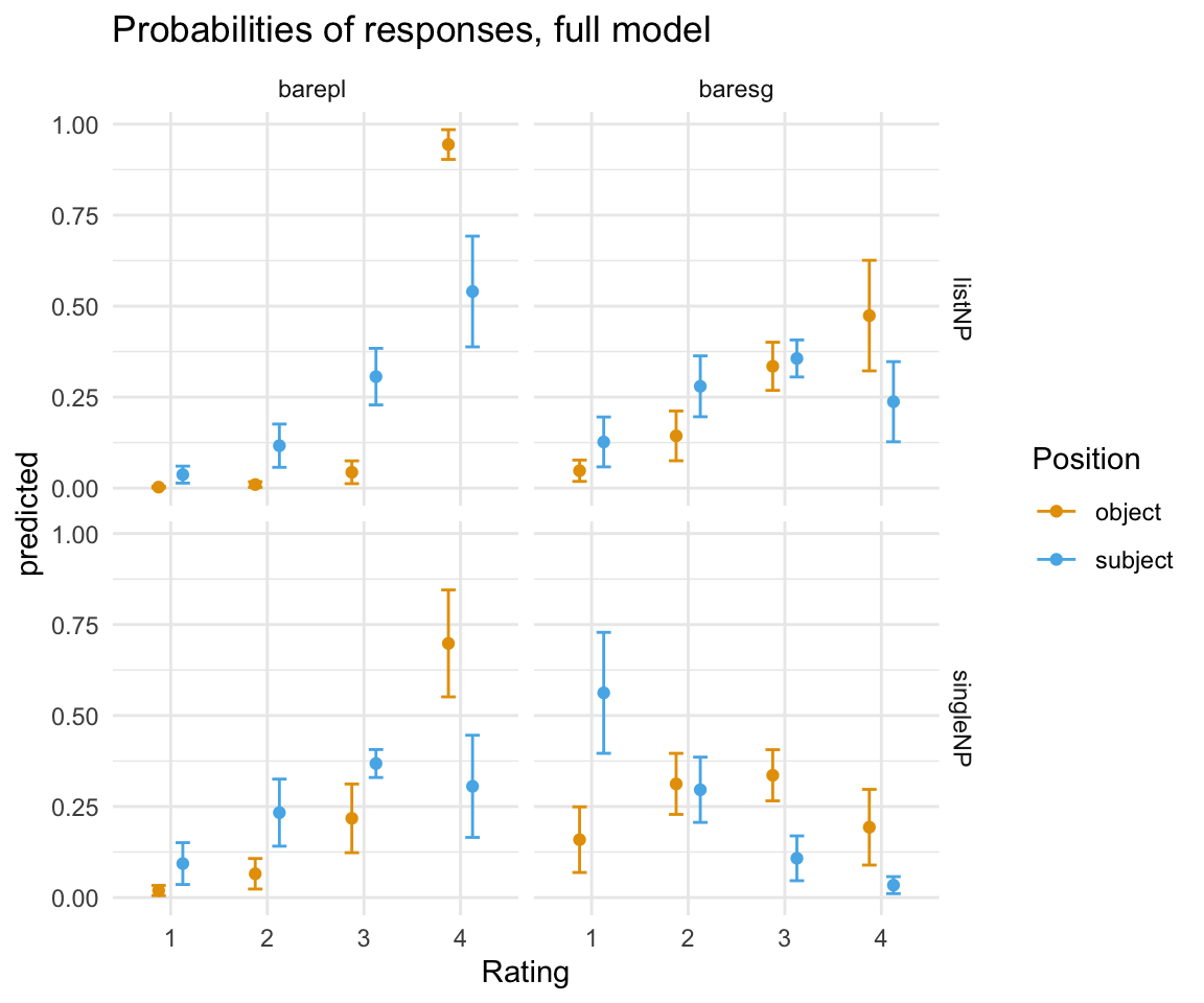
ggplot(ggpredictions_ols6, aes(x = Position, y = predicted, fill = Rating)) + geom_bar(position = "dodge", stat = "identity") + facet_grid(survey~NP) + scale_fill_manual(values = cbPalette) + theme_minimal()+ ggtitle("Probabilities of responses, full model")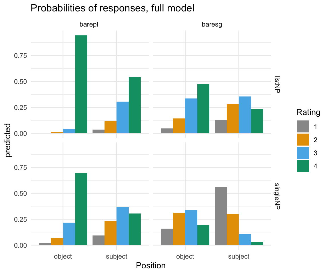
ggpredictions_ols6 %>% mutate(Rating = ordered(Rating, levels=rev(levels(Rating)))) %>% ggplot( aes(x = Position, y = predicted, fill = Rating)) + geom_bar(position = "fill", stat = "identity") + facet_grid(survey~NP) + scale_fill_manual(values = cbPalette) + theme_minimal() + ggtitle("Probabilities of responses, full model (reversed color scheme)")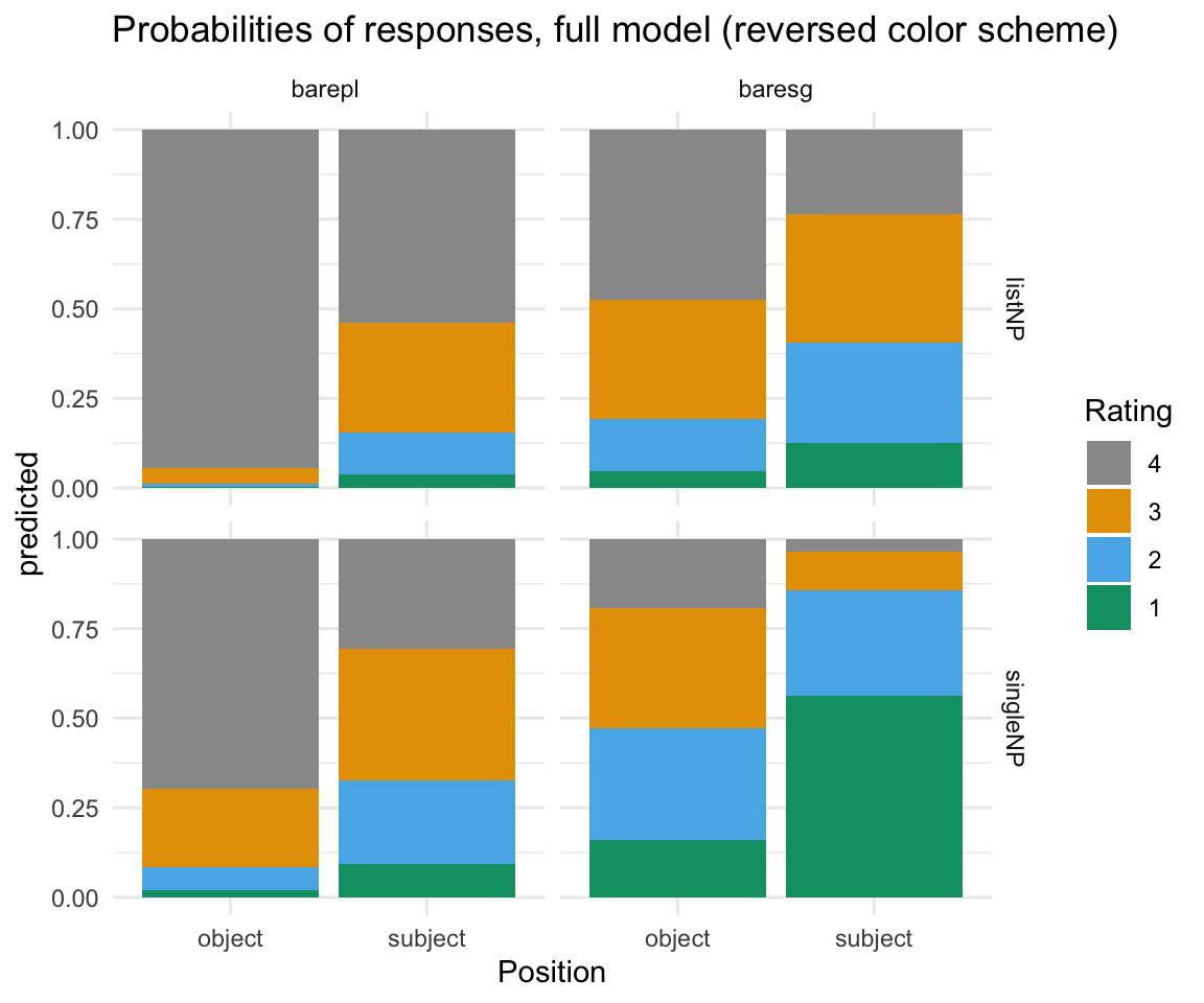
ggplot(ggpredictions_ols6, aes(x = Position, y = predicted, fill = Rating)) + geom_bar(position = "fill", stat = "identity") + facet_grid(survey~NP) + scale_fill_manual(values = cbPalette) + theme_minimal() + ggtitle("Probabilities of responses, full model")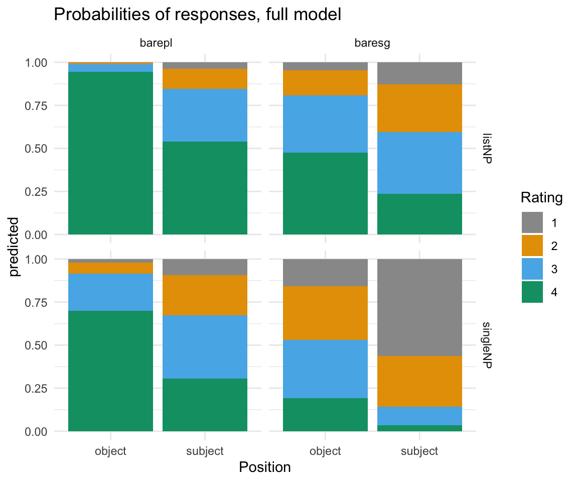
Questions?