GAM in R
Packages
The packages you will need for this workshop are as follows. I am also including the hex codes for a colorblind-friendly palette, which I use for my plots. I used the gganimate package to show my dissertation data (below), but this is not crucial for data processing/analysis.
library(tidyverse)
library(mgcv)
library(itsadug)
library(mgcViz)
cbPalette <- c("#999999", "#E69F00", "#56B4E9", "#009E73", "#F0E442", "#0072B2", "#D55E00", "#CC79A7")
Data
The data I am using in this workshop is my dissertation acoustics data. A copy can be found here. The data has the following variables:
- Speaker
- Vowel
- Nasality
- Repetiton Number
- Normalized Time
- F1
- F2
- F3
- F3-F2 difference
## Parsed with column specification:
## cols(
##   Speaker = col_character(),
##   Word = col_character(),
##   Vowel = col_character(),
##   Nasality = col_character(),
##   RepNo = col_double(),
##   NormTime = col_double(),
##   Type = col_character(),
##   label = col_character(),
##   Time = col_double(),
##   F1 = col_double(),
##   F2 = col_double(),
##   F3 = col_double(),
##   F2_3 = col_double()
## )
head(normtimeBP) ## # A tibble: 6 x 9
## # Groups: Speaker [1]
## Speaker Vowel Nasality RepNo NormTime F1 F2 F3 F2_3
## <fct> <fct> <fct> <fct> <dbl> <dbl> <dbl> <dbl> <dbl>
## 1 BP02 u nasal 1 0.1 569. 2372. 3130. 379.
## 2 BP02 u nasal 1 0.2 364. 2297. 2692. 197.
## 3 BP02 u nasal 1 0.3 373. 2258. 2882. 312.
## 4 BP02 u nasal 1 0.4 303. 2165. 2918. 376.
## 5 BP02 u nasal 1 0.5 415. 2247. 2893. 323.
## 6 BP02 u nasal 1 0.6 336. 2098. 2623. 263.str(normtimeBP, give.attr = FALSE)## tibble [46,876 × 9] (S3: grouped_df/tbl_df/tbl/data.frame)
## $ Speaker : Factor w/ 12 levels "BP02","BP04",..: 1 1 1 1 1 1 1 1 1 1 ...
## $ Vowel : Factor w/ 3 levels "a","i","u": 3 3 3 3 3 3 3 3 3 3 ...
## $ Nasality: Factor w/ 4 levels "nasal","nasal_final",..: 1 1 1 1 1 1 1 1 1 1 ...
## $ RepNo : Factor w/ 70 levels "1","2","3","4",..: 1 1 1 1 1 1 1 1 1 1 ...
## $ NormTime: num [1:46876] 0.1 0.2 0.3 0.4 0.5 0.6 0.7 0.8 0.9 1 ...
## $ F1 : num [1:46876] 569 364 373 303 415 ...
## $ F2 : num [1:46876] 2372 2297 2258 2165 2247 ...
## $ F3 : num [1:46876] 3130 2692 2882 2918 2893 ...
## $ F2_3 : num [1:46876] 379 197 312 376 323 ...dim(normtimeBP)## [1] 46876 9levels(normtimeBP$Nasality)## [1] "nasal" "nasal_final" "nasalized" "oral"animate(BP02_animation, height=450, width = 450)
What is a generalized additive model?
A generalized additive model (henceforth, GAM) is a model that relaxes the assumption of a linear relaiton between the dependent variable and a predictor or set of predictors. The relationship between dependent and independent variables is instead estimated by a smooth function, which is created by an addition (hence additive model!) of multiple basis functions.
GAM has a number of advantages over linear and polynomial regressions. For instance, the optimal shape of the non-linearity is determined automatically by the model, as opposed to comparing various shapes of models. The appropriate smoothness is determined by combining calculations for minimizations of error in addition to penalizing “wiggliness” of the model. This combination of error minimization and non-linearity penalty is done in order to avoid overfitting.GAM models non-linearities by incorporating one or more smooths of predictor variables, which have their own basis functions. The basic smooth in a GAM is a thin plate regression spline, which combines increasingly complex basis functions. GAM also allows for multiple dimensions of a predictor to be incorporated onto a (hyper) surface smooth.
Running a GAM in R
Fitting a basic GAM
The first GAM I am going to fit looks at differences in F1 for different nasality conditions. For this particular question, I will begin by looking only at one speaker’s data, and only at the vowel /a/.
What does this mean? The output should look quite similar to that of a linear (mixed effects) model.
BP02a = normtimeBP%>% filter(Speaker=="BP02"& Vowel=="a")

BP02gam1 = gam(F1~Nasality, data = BP02a)
summary(BP02gam1)
##
## Family: gaussian
## Link function: identity
##
## Formula:
## F1 ~ Nasality
##
## Parametric coefficients:
## Estimate Std. Error t value Pr(>|t|)
## (Intercept) 358.257 4.634 77.32 <2e-16 ***
## Nasalitynasalized 131.894 6.592 20.01 <2e-16 ***
## Nasalityoral 321.441 6.831 47.05 <2e-16 ***
## ---
## Signif. codes: 0 '***' 0.001 '**' 0.01 '*' 0.05 '.' 0.1 ' ' 1
##
##
## R-sq.(adj) = 0.699 Deviance explained = 70%
## GCV = 7279.5 Scale est. = 7256.7 n = 956Now, let’s add in a smooth term. This is a thin plate regression spline, where we are smoothing over time.
BP02gam2 = gam(F1~Nasality + s(NormTime), data = BP02a)
summary(BP02gam2)
##
## Family: gaussian
## Link function: identity
##
## Formula:
## F1 ~ Nasality + s(NormTime)
##
## Parametric coefficients:
## Estimate Std. Error t value Pr(>|t|)
## (Intercept) 357.859 3.419 104.68 <2e-16 ***
## Nasalitynasalized 131.831 4.864 27.11 <2e-16 ***
## Nasalityoral 322.833 5.042 64.03 <2e-16 ***
## ---
## Signif. codes: 0 '***' 0.001 '**' 0.01 '*' 0.05 '.' 0.1 ' ' 1
##
## Approximate significance of smooth terms:
## edf Ref.df F p-value
## s(NormTime) 6.693 7.846 101.5 <2e-16 ***
## ---
## Signif. codes: 0 '***' 0.001 '**' 0.01 '*' 0.05 '.' 0.1 ' ' 1
##
## R-sq.(adj) = 0.836 Deviance explained = 83.8%
## GCV = 3989.9 Scale est. = 3949.5 n = 956What do we have here? We have two sections of the model - parametric coefficients, and non-parametric coefficients.
Let’s go over the following:
- Meaning of parametric coefficients
- Meaning of non-parametric coefficients
- Model statistics (Deviance explained, etc.)
- Effective degrees of freedom
What if we want to add in time dynamics separately for each nasality condition? Let’s build a third model:
BP02gam3 = gam(F1~ Nasality + s(NormTime, by = Nasality), data = BP02a)
summary(BP02gam3)
##
## Family: gaussian
## Link function: identity
##
## Formula:
## F1 ~ Nasality + s(NormTime, by = Nasality)
##
## Parametric coefficients:
## Estimate Std. Error t value Pr(>|t|)
## (Intercept) 358.481 1.847 194.04 <2e-16 ***
## Nasalitynasalized 131.150 2.629 49.89 <2e-16 ***
## Nasalityoral 324.388 2.726 119.00 <2e-16 ***
## ---
## Signif. codes: 0 '***' 0.001 '**' 0.01 '*' 0.05 '.' 0.1 ' ' 1
##
## Approximate significance of smooth terms:
## edf Ref.df F p-value
## s(NormTime):Nasalitynasal 6.513 7.686 215.5 <2e-16 ***
## s(NormTime):Nasalitynasalized 7.544 8.497 59.9 <2e-16 ***
## s(NormTime):Nasalityoral 7.048 8.136 352.6 <2e-16 ***
## ---
## Signif. codes: 0 '***' 0.001 '**' 0.01 '*' 0.05 '.' 0.1 ' ' 1
##
## R-sq.(adj) = 0.952 Deviance explained = 95.3%
## GCV = 1183 Scale est. = 1153.1 n = 956Visualizing GAM results
GAM interpretation relies heavily on visualization. There are a number of methods available for plotting GAM results. One is to use the plot function in R, which passes your model to plot.GAM. Note the difference between plotting the fits for these two models.
plot(BP02gam2)
plot(BP02gam3, pages = 1)
Another method for plotting GAM results is the mgcViz package. This package utilizes ggplot2 as a plotting basis, which allows customization of plots. In order to utilize this package, the visualization of a model needs to be extracted, and then the model can be plotted.
BP02gam3viz = getViz(BP02gam3, nsim = 0)
print(plot(BP02gam3viz), pages = 1)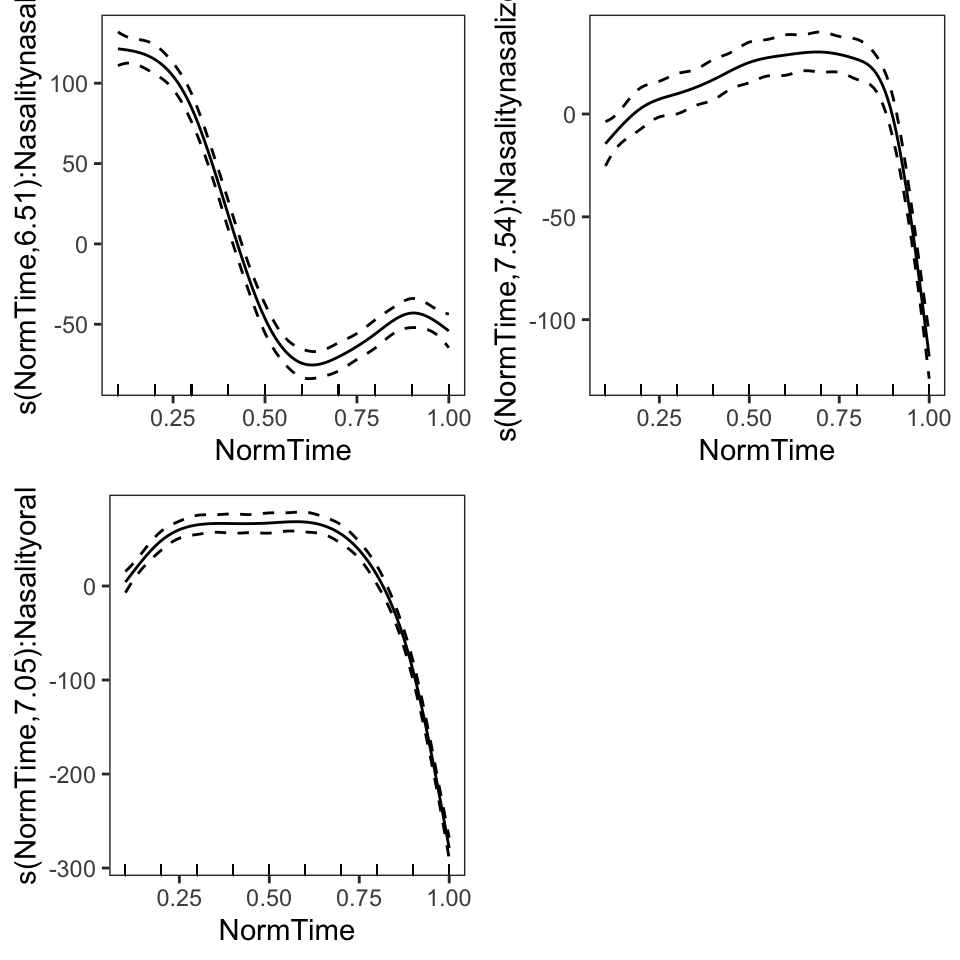
The method that has been adopted for plotting is using the itsadug package, which was actually developed in part by linguists. The itsadug package allows for plotting of different smooths, as well as differences between conditions.
We will go through how to plot results of a gam using the plot_smooth and plot_diff functions. Note the difference between plotting the model without and with individual smooths by Nasality.
We will begin by using the plot_smooth() function. This takes the following arguments:
- model name
- view (name of your smoothed independent x-axis variable)
- cond (named list of the values to use for the other predictor terms) OR plot_all (vector with the name(s) of model predictors, for which all levels should be plotted)
- rm.ranef (whether or not to remove random effects, if they are included in the model. Default is TRUE)
- Other plotting specifications (xlab, ylab, xlim, ylim, col, main, etc.)
We will then use the plot_diff() function, which plots a difference curve based on model predictions. The plot_diff() function takes the following arguments:
- model name
- view (name of your smoothed independent x-axis variable)
- comp (list of the grouping predictor variable, and the two levels of this variable to calculate the difference for)
- cond (named list of the values to use for the other predictor terms) OR plot_all (vector with the name(s) of model predictors, for which all levels should be plotted)
- rm.ranef (whether or not to remove random effects, if they are included in the model. Default is TRUE)
- Other plotting specifications (xlab, ylab, xlim, ylim, col, main, etc.)
Note that these plotting methods in itsadug are plotting summed effects. That is, it is plotting the smooth of the different conditions, with a constant y-axis shift of the parametric coefficients.
par(mfrow = c(2,2))
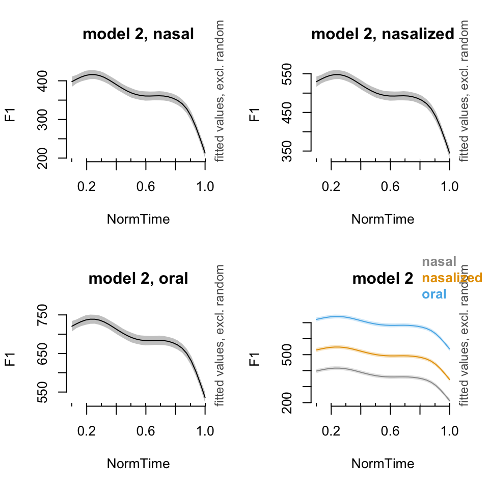
#Model 2: Without different smooths for nasality
plot_smooth(BP02gam2, view = "NormTime", cond = list(Nasality = "nasal"), main = "model 2, nasal")## Summary:
## * Nasality : factor; set to the value(s): nasal.
## * NormTime : numeric predictor; with 30 values ranging from 0.100000 to 1.000000.
## * NOTE : No random effects in the model to cancel.
## plot_smooth(BP02gam2, view = "NormTime", cond = list(Nasality = "nasalized"), main = "model 2, nasalized")## Summary:
## * Nasality : factor; set to the value(s): nasalized.
## * NormTime : numeric predictor; with 30 values ranging from 0.100000 to 1.000000.
## * NOTE : No random effects in the model to cancel.
## plot_smooth(BP02gam2, view = "NormTime", cond = list(Nasality = "oral"), main = "model 2, oral")## Summary:
## * Nasality : factor; set to the value(s): oral.
## * NormTime : numeric predictor; with 30 values ranging from 0.100000 to 1.000000.
## * NOTE : No random effects in the model to cancel.
## plot_smooth(BP02gam2, view = "NormTime", plot_all = c("Nasality"), main = "model 2", col = cbPalette[1:3])## Summary:
## * Nasality : factor; set to the value(s): nasal, nasalized, oral.
## * NormTime : numeric predictor; with 30 values ranging from 0.100000 to 1.000000.
## * NOTE : No random effects in the model to cancel.
## 
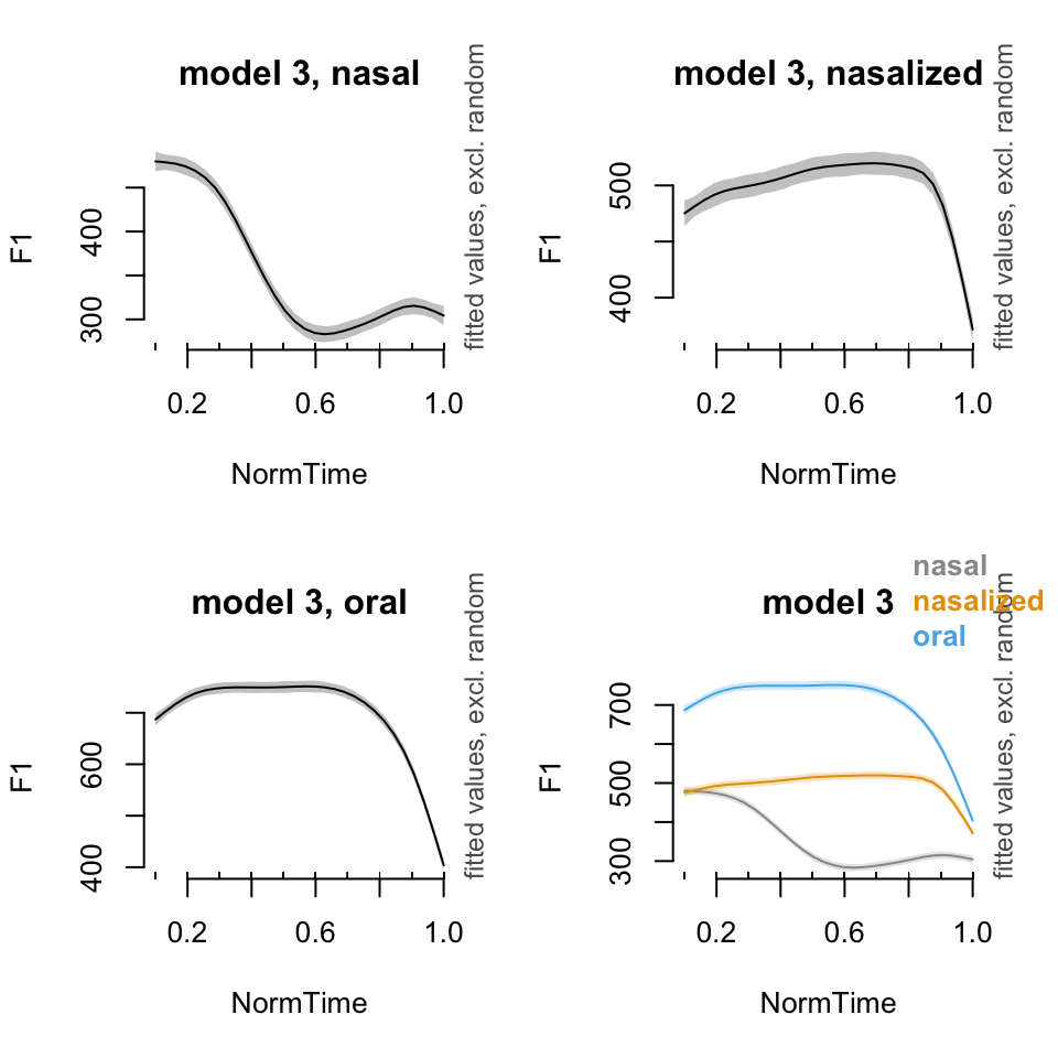
#Model 3: With different smooths for nasality

plot_smooth(BP02gam3, view = "NormTime", cond = list(Nasality = "nasal"), main = "model 3, nasal")
## Summary:
## * Nasality : factor; set to the value(s): nasal.
## * NormTime : numeric predictor; with 30 values ranging from 0.100000 to 1.000000.
## * NOTE : No random effects in the model to cancel.
## plot_smooth(BP02gam3, view = "NormTime", cond = list(Nasality = "nasalized"), main = "model 3, nasalized")## Summary:
## * Nasality : factor; set to the value(s): nasalized.
## * NormTime : numeric predictor; with 30 values ranging from 0.100000 to 1.000000.
## * NOTE : No random effects in the model to cancel.
## plot_smooth(BP02gam3, view = "NormTime", cond = list(Nasality = "oral"), main = "model 3, oral")## Summary:
## * Nasality : factor; set to the value(s): oral.
## * NormTime : numeric predictor; with 30 values ranging from 0.100000 to 1.000000.
## * NOTE : No random effects in the model to cancel.
## plot_smooth(BP02gam3, view = "NormTime", plot_all = c("Nasality"), main = "model 3", col = cbPalette[1:3])## Summary:
## * Nasality : factor; set to the value(s): nasal, nasalized, oral.
## * NormTime : numeric predictor; with 30 values ranging from 0.100000 to 1.000000.
## * NOTE : No random effects in the model to cancel.
## 
par(mfrow = c(1, 1))
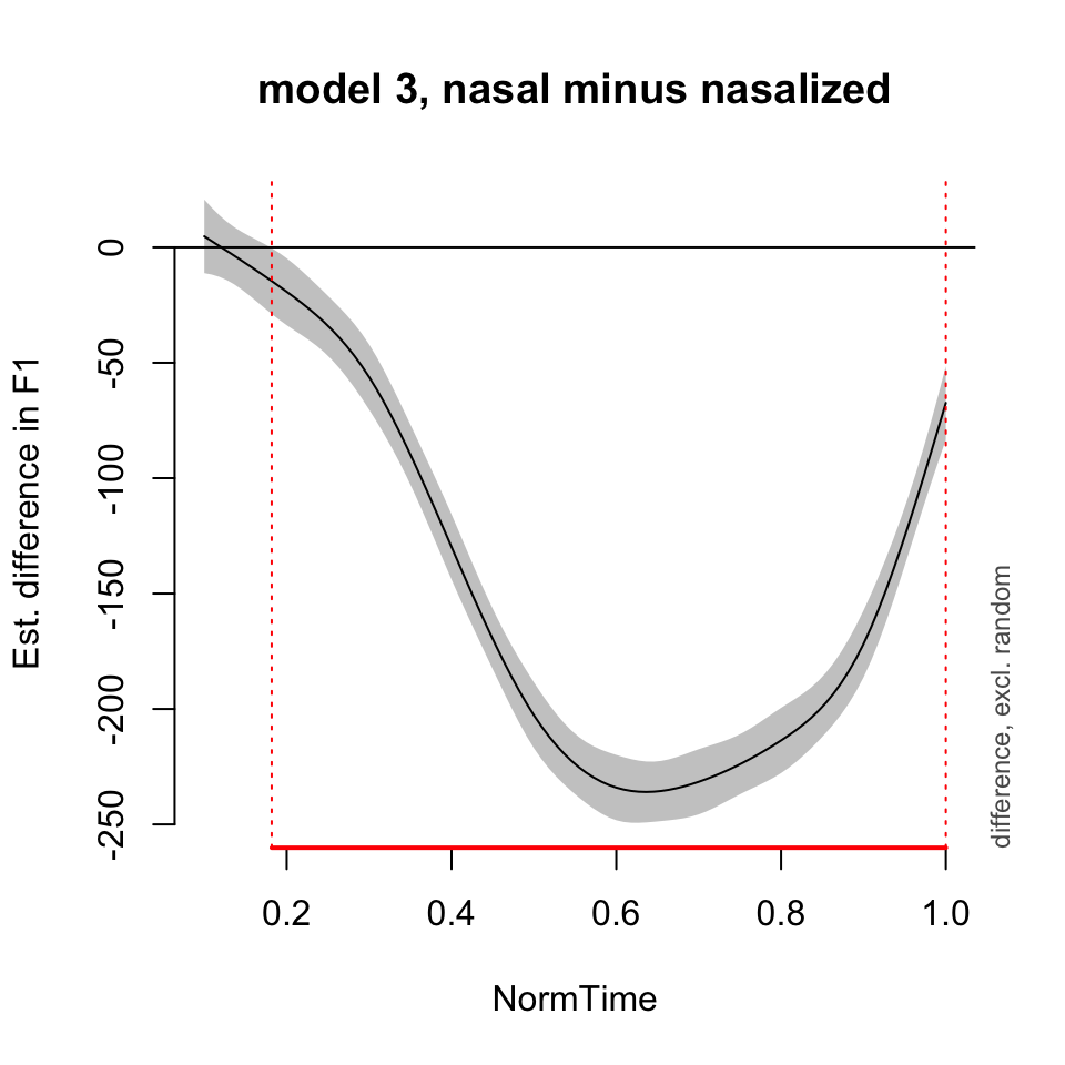
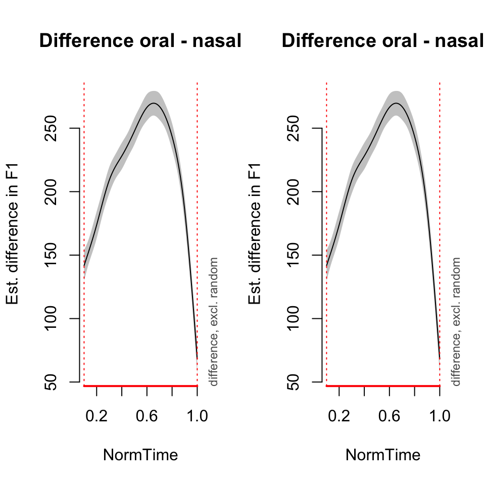
plot_diff(BP02gam3, view = "NormTime", comp = list(Nasality = c("nasal", "nasalized")), main = "model 3, nasal minus nasalized")## Summary:
## * NormTime : numeric predictor; with 100 values ranging from 0.100000 to 1.000000.
## * NOTE : No random effects in the model to cancel.
## 
##
## NormTime window(s) of significant difference(s):
##  0.181818 - 1.000000
Random effects
Recall that fixed effects factors are categorical, with a small number of levels, all of which are included in our data and are used to answer a research question. Random effects, on the other hand, introduce systematic variation into the model. There are generally a larger number of categorical levels, and we are generally interested in generalizing over these levels. These levels are generally sampled from a larger population.
Random intercepts
Random intercepts allow for differences in the “baseline” across all levels of a random effect. However, the relationship between the predictor and the response variables maintains the same structure - they are just shifted up or down along the y-axis. Hence, the intercept of the line differs for each participant/word/other random variable.
In lme4, a random intercept is included with the syntax (1|Participant) (where participant is the random effect in question). In mgcv, a random intercept is included with the syntax s(Participant, bs=“re”). Here, participant is the random effect, and bs=“re” tells R that the basis function here is a random effect structure.
Let’s build a model with a random intercept, and show how to interpret it and plot the results. First, there is a model run with no random effect, then a model with a random intercept. First, notice the differences in the summaries of these models. Then, is there a difference in deviance explained?
Here, I am including only a subset of the speakers from my dataset, because otherwise it takes forever to compile this document!
BPa = normtimeBP%>% filter(Vowel=="a", Speaker %in% c("BP02", "BP04", "BP05", "BP10", "BP14"))
BPgama0 = gam(F1~ Nasality + s(NormTime, by = Nasality) , data = BPa, method = "REML")
summary(BPgama0)
##
## Family: gaussian
## Link function: identity
##
## Formula:
## F1 ~ Nasality + s(NormTime, by = Nasality)
##
## Parametric coefficients:
## Estimate Std. Error t value Pr(>|t|)
## (Intercept) 374.497 1.558 240.38 <2e-16 ***
## Nasalitynasalized 46.917 2.217 21.16 <2e-16 ***
## Nasalityoral 201.992 2.209 91.45 <2e-16 ***
## ---
## Signif. codes: 0 '***' 0.001 '**' 0.01 '*' 0.05 '.' 0.1 ' ' 1
##
## Approximate significance of smooth terms:
## edf Ref.df F p-value
## s(NormTime):Nasalitynasal 4.181 5.159 229.94 <2e-16 ***
## s(NormTime):Nasalitynasalized 5.160 6.294 32.99 <2e-16 ***
## s(NormTime):Nasalityoral 7.576 8.517 361.24 <2e-16 ***
## ---
## Signif. codes: 0 '***' 0.001 '**' 0.01 '*' 0.05 '.' 0.1 ' ' 1
##
## R-sq.(adj) = 0.66 Deviance explained = 66.1%
## -REML = 40153 Scale est. = 5718.3 n = 6988BPgama1 = gam(F1~ Nasality + s(NormTime, by = Nasality) + s(Speaker, bs = "re"), data = BPa, method = "REML")
summary(BPgama1)##
## Family: gaussian
## Link function: identity
##
## Formula:
## F1 ~ Nasality + s(NormTime, by = Nasality) + s(Speaker, bs = "re")
##
## Parametric coefficients:
## Estimate Std. Error t value Pr(>|t|)
## (Intercept) 376.576 13.662 27.57 <2e-16 ***
## Nasalitynasalized 46.979 2.105 22.32 <2e-16 ***
## Nasalityoral 203.208 2.098 96.86 <2e-16 ***
## ---
## Signif. codes: 0 '***' 0.001 '**' 0.01 '*' 0.05 '.' 0.1 ' ' 1
##
## Approximate significance of smooth terms:
## edf Ref.df F p-value
## s(NormTime):Nasalitynasal 4.317 5.321 247.49 <2e-16 ***
## s(NormTime):Nasalitynasalized 5.320 6.472 35.59 <2e-16 ***
## s(NormTime):Nasalityoral 7.692 8.588 402.36 <2e-16 ***
## s(Speaker) 3.983 4.000 189.74 <2e-16 ***
## ---
## Signif. codes: 0 '***' 0.001 '**' 0.01 '*' 0.05 '.' 0.1 ' ' 1
##
## R-sq.(adj) = 0.694 Deviance explained = 69.5%
## -REML = 39804 Scale est. = 5156.4 n = 6988As you can see, there is a difference in deviance explained, as well as in the summary - there is an extra line in the smooth terms for s(Speaker).
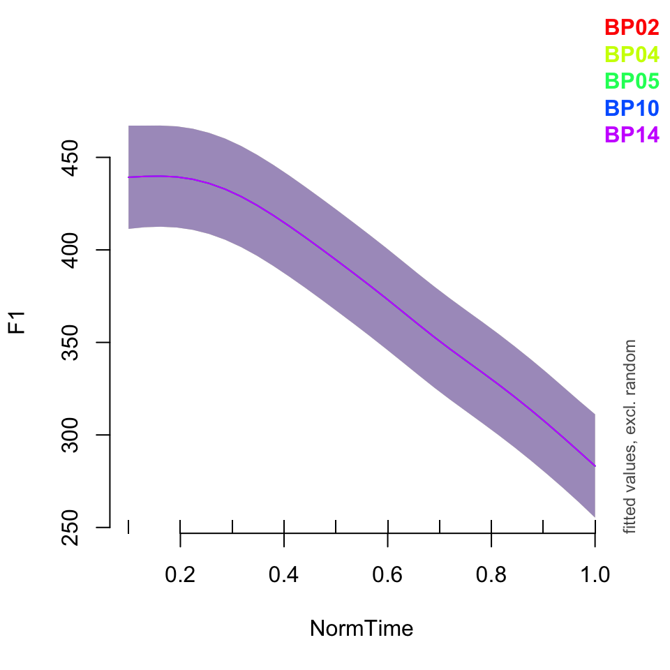
Now, let’s talk about visualization of these terms. Let’s first visualize the fit for nasal /a/, for the models with and without random term. What is the default setting for the model with the random effect?
plot_smooth(BPgama0, view = "NormTime", cond = list(Nasality = "nasal"))## Summary:
## * Nasality : factor; set to the value(s): nasal.
## * NormTime : numeric predictor; with 30 values ranging from 0.100000 to 1.000000.
## * NOTE : No random effects in the model to cancel.
## 
plot_smooth(BPgama1, view = "NormTime", cond = list(Nasality = "nasal"))## Summary:
## * Nasality : factor; set to the value(s): nasal.
## * NormTime : numeric predictor; with 30 values ranging from 0.100000 to 1.000000.
## * Speaker : factor; set to the value(s): BP04. (Might be canceled as random effect, check below.)
## * NOTE : The following random effects columns are canceled: s(Speaker)
## 
As you can see, the models look pretty similar, except for model BPgama1, the plot is set to Speaker = “BP04”. What if we wanted to see another speaker’s data?
plot_smooth(BPgama1, view = "NormTime", cond = list(Nasality = "nasal", Speaker = "BP10"))## Summary:
## * Nasality : factor; set to the value(s): nasal.
## * NormTime : numeric predictor; with 30 values ranging from 0.100000 to 1.000000.
## * Speaker : factor; set to the value(s): BP10. (Might be canceled as random effect, check below.)
## * NOTE : The following random effects columns are canceled: s(Speaker)
## 
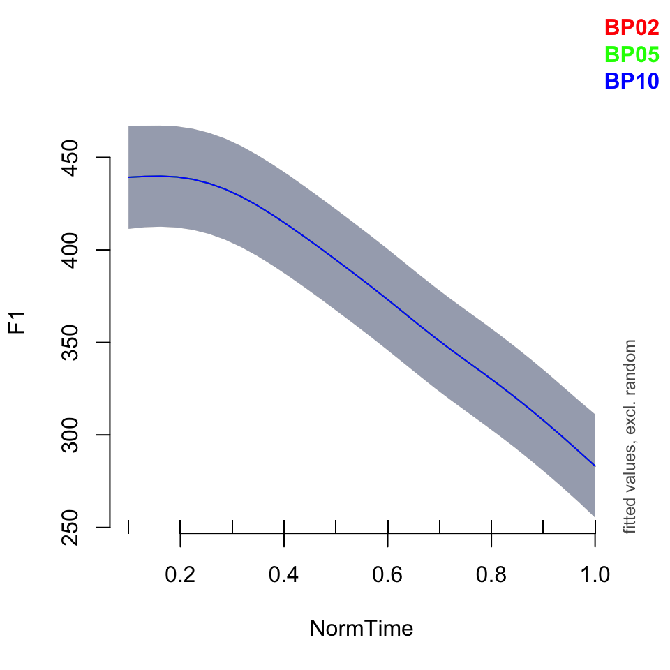
What if we wanted to plot the data for a few speakers? Or all of them? If you would like to plot only a subset of your speakers, you need to specify that you want to plot “all” speakers, then list the ones you want to plot specifically.
Notice that the relationship between time and F1 is the same for all speakers - just the baseline has been moved up or down!
plot_smooth(BPgama1, view = "NormTime", cond = list(Nasality = "nasal"), plot_all = "Speaker")## Summary:
## * Nasality : factor; set to the value(s): nasal.
## * NormTime : numeric predictor; with 30 values ranging from 0.100000 to 1.000000.
## * Speaker : factor; set to the value(s): BP02, BP04, BP05, BP10, BP14. (Might be canceled as random effect, check below.)
## * NOTE : The following random effects columns are canceled: s(Speaker)
## 
plot_smooth(BPgama1, view = "NormTime", cond = list(Nasality = "nasal",Speaker = c("BP02", "BP05", "BP10")), plot_all = "Speaker")## Warning in plot_smooth(BPgama1, view = "NormTime", cond = list(Nasality =
## "nasal", : Speaker in cond and in plot_all. Not all levels are being plotted.## Summary:
## * Nasality : factor; set to the value(s): nasal.
## * NormTime : numeric predictor; with 30 values ranging from 0.100000 to 1.000000.
## * Speaker : factor; set to the value(s): BP02, BP05, BP10. (Might be canceled as random effect, check below.)
## * NOTE : The following random effects columns are canceled: s(Speaker)
## 
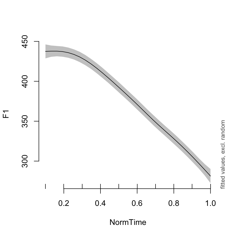
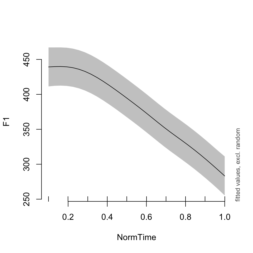
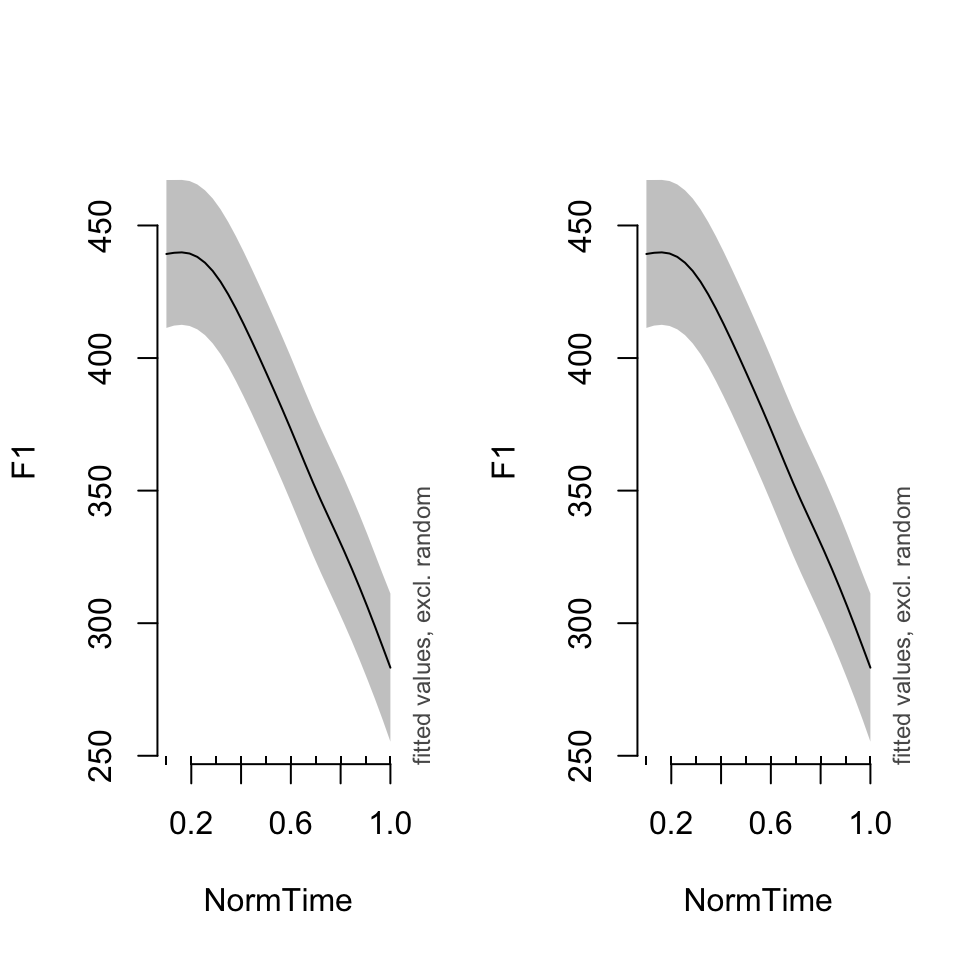
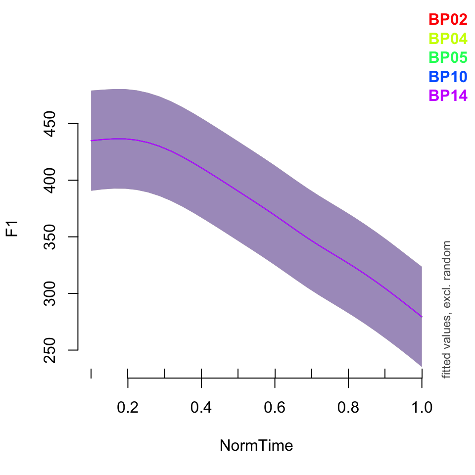
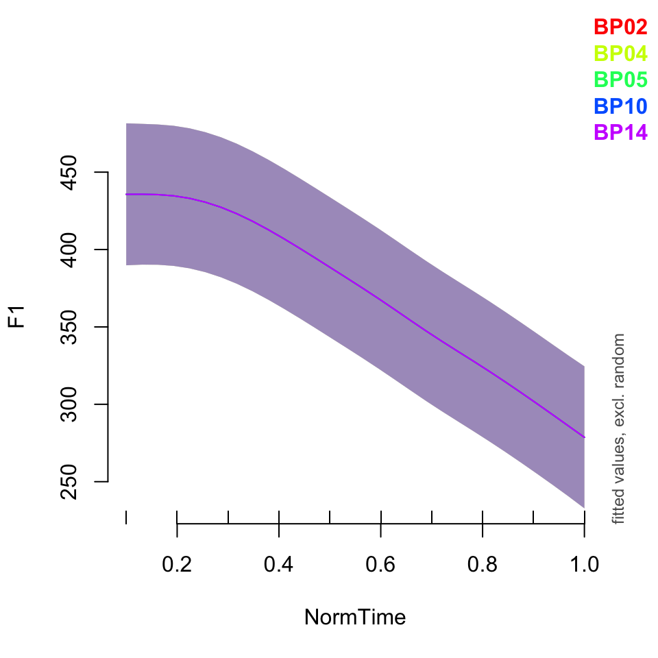
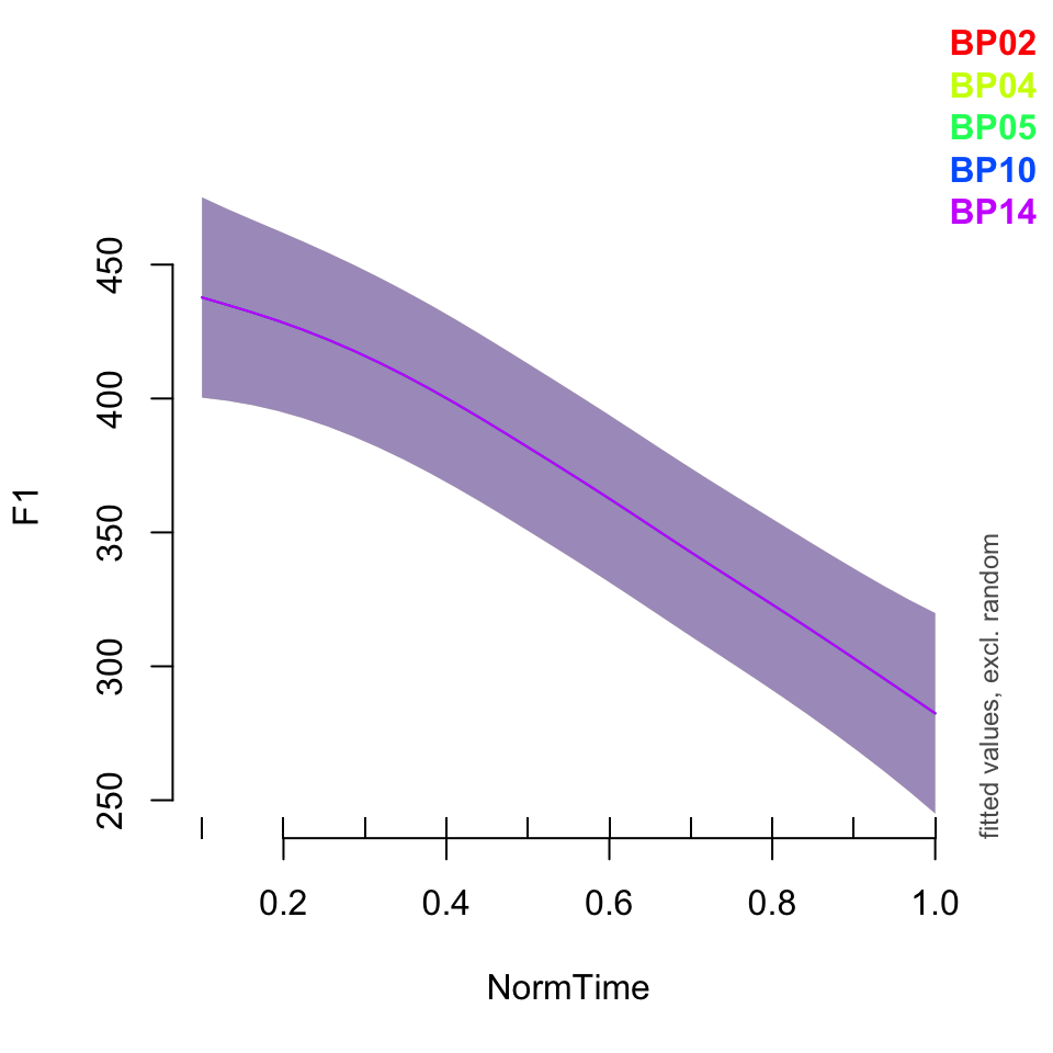
What if we wanted to see the overall trend, rather than a particular speaker’s data? In both plot_smooth() and plot_diff(), you can use rm.ranef = TRUE to show the overall shape of the model. Notice the difference in the size of the confidence intervals.
par(mfrow = c(1,2))
plot_smooth(BPgama1, view = "NormTime", cond = list(Nasality = "nasal"))## Summary:
## * Nasality : factor; set to the value(s): nasal.
## * NormTime : numeric predictor; with 30 values ranging from 0.100000 to 1.000000.
## * Speaker : factor; set to the value(s): BP04. (Might be canceled as random effect, check below.)
## * NOTE : The following random effects columns are canceled: s(Speaker)
## plot_smooth(BPgama1, view = "NormTime", cond = list(Nasality = "nasal"), rm.ranef = TRUE)## Summary:
## * Nasality : factor; set to the value(s): nasal.
## * NormTime : numeric predictor; with 30 values ranging from 0.100000 to 1.000000.
## * Speaker : factor; set to the value(s): BP04. (Might be canceled as random effect, check below.)
## * NOTE : The following random effects columns are canceled: s(Speaker)
## 
plot_diff(BPgama1, view = "NormTime", comp = list(Nasality =c("oral", "nasal")))## Summary:
## * NormTime : numeric predictor; with 100 values ranging from 0.100000 to 1.000000.
## * Speaker : factor; set to the value(s): BP04. (Might be canceled as random effect, check below.)
## * NOTE : The following random effects columns are canceled: s(Speaker)
## ##
## NormTime window(s) of significant difference(s):
## 0.100000 - 1.000000plot_diff(BPgama1, view = "NormTime", comp = list(Nasality =c("oral", "nasal")), rm.ranef = TRUE)## Summary:
## * NormTime : numeric predictor; with 100 values ranging from 0.100000 to 1.000000.
## * Speaker : factor; set to the value(s): BP04. (Might be canceled as random effect, check below.)
## * NOTE : The following random effects columns are canceled: s(Speaker)
## 
##
## NormTime window(s) of significant difference(s):
## 0.100000 - 1.000000par(mfrow = c(1,1))Random slopes
Random slopes allow for differences in the relationship between a predictor variable and the response variable, for each level of the random effect. These are often used if there are possible individual differences in these relationships, which could have an influence on the model. For example, differences in anatomical structure could lead to differences in vowel space (i.e. the distance in F1 between /a/ and /i/ could be bigger for a male speaker, due to having a larger oral cavity). Or, there could be social influences on the magnitude of the difference between oral and nasal vowels. Therefore, random slopes should be used.
In lme4, a random slope with correlated random intercept is included with the syntax (1+Nasality|Participant), and a random slope with no variation in intercept is included with the syntax (0+Nasality|Participant) where participant is the random effect in question, and the random slope is built for each level of Nasality). In mgcv, a random slope is included with the syntax s(Participant,Nasality, bs=“re”). Here, participant is the random effect, the random slope is being built over Nasality, and bs=“re” tells R that the basis function here is a random effect structure. Note that this is the analog of (0+Nasality|Participant) for lme4 syntax. The structure (1+Nasality|Participant) is not possible in mgcv, so a random slope and random intercept must be specified.
First, what is the difference in these models, and their summaries?
BPgama1 = gam(F1~ Nasality + s(NormTime, by = Nasality) + s(Speaker, bs = "re"), data = BPa, method = "REML")
summary(BPgama1)
##
## Family: gaussian
## Link function: identity
##
## Formula:
## F1 ~ Nasality + s(NormTime, by = Nasality) + s(Speaker, bs = "re")
##
## Parametric coefficients:
## Estimate Std. Error t value Pr(>|t|)
## (Intercept) 376.576 13.662 27.57 <2e-16 ***
## Nasalitynasalized 46.979 2.105 22.32 <2e-16 ***
## Nasalityoral 203.208 2.098 96.86 <2e-16 ***
## ---
## Signif. codes: 0 '***' 0.001 '**' 0.01 '*' 0.05 '.' 0.1 ' ' 1
##
## Approximate significance of smooth terms:
## edf Ref.df F p-value
## s(NormTime):Nasalitynasal 4.317 5.321 247.49 <2e-16 ***
## s(NormTime):Nasalitynasalized 5.320 6.472 35.59 <2e-16 ***
## s(NormTime):Nasalityoral 7.692 8.588 402.36 <2e-16 ***
## s(Speaker) 3.983 4.000 189.74 <2e-16 ***
## ---
## Signif. codes: 0 '***' 0.001 '**' 0.01 '*' 0.05 '.' 0.1 ' ' 1
##
## R-sq.(adj) = 0.694 Deviance explained = 69.5%
## -REML = 39804 Scale est. = 5156.4 n = 6988BPgama2 = gam(F1~ Nasality + s(NormTime, by = Nasality)+ s(Speaker, Nasality, bs = "re"), data = BPa, method = "REML")
summary(BPgama2)##
## Family: gaussian
## Link function: identity
##
## Formula:
## F1 ~ Nasality + s(NormTime, by = Nasality) + s(Speaker, Nasality,
## bs = "re")
##
## Parametric coefficients:
## Estimate Std. Error t value Pr(>|t|)
## (Intercept) 372.83 22.28 16.732 < 2e-16 ***
## Nasalitynasalized 51.05 31.51 1.620 0.105
## Nasalityoral 211.98 31.51 6.727 1.87e-11 ***
## ---
## Signif. codes: 0 '***' 0.001 '**' 0.01 '*' 0.05 '.' 0.1 ' ' 1
##
## Approximate significance of smooth terms:
## edf Ref.df F p-value
## s(NormTime):Nasalitynasal 4.715 5.787 285.48 <2e-16 ***
## s(NormTime):Nasalitynasalized 5.654 6.833 42.75 <2e-16 ***
## s(NormTime):Nasalityoral 7.909 8.706 503.12 <2e-16 ***
## s(Speaker,Nasality) 11.955 12.000 225.29 <2e-16 ***
## ---
## Signif. codes: 0 '***' 0.001 '**' 0.01 '*' 0.05 '.' 0.1 ' ' 1
##
## R-sq.(adj) = 0.755 Deviance explained = 75.6%
## -REML = 39044 Scale est. = 4119.1 n = 6988BPgama3 = gam(F1~ Nasality + s(NormTime, by = Nasality) + s(Speaker, bs = "re")+ s(Speaker, Nasality, bs = "re"), data = BPa, method = "REML")
summary(BPgama3)##
## Family: gaussian
## Link function: identity
##
## Formula:
## F1 ~ Nasality + s(NormTime, by = Nasality) + s(Speaker, bs = "re") +
## s(Speaker, Nasality, bs = "re")
##
## Parametric coefficients:
## Estimate Std. Error t value Pr(>|t|)
## (Intercept) 372.83 22.28 16.733 < 2e-16 ***
## Nasalitynasalized 51.05 31.51 1.620 0.105
## Nasalityoral 211.98 31.51 6.728 1.86e-11 ***
## ---
## Signif. codes: 0 '***' 0.001 '**' 0.01 '*' 0.05 '.' 0.1 ' ' 1
##
## Approximate significance of smooth terms:
## edf Ref.df F p-value
## s(NormTime):Nasalitynasal 4.714905 5.787 285.490 <2e-16 ***
## s(NormTime):Nasalitynasalized 5.653945 6.833 42.747 <2e-16 ***
## s(NormTime):Nasalityoral 7.908816 8.706 503.121 <2e-16 ***
## s(Speaker) 0.003491 4.000 0.041 0.581
## s(Speaker,Nasality) 11.951036 12.000 239.903 <2e-16 ***
## ---
## Signif. codes: 0 '***' 0.001 '**' 0.01 '*' 0.05 '.' 0.1 ' ' 1
##
## R-sq.(adj) = 0.755 Deviance explained = 75.6%
## -REML = 39044 Scale est. = 4119.1 n = 6988Next, let’s look at all of the speakers’ data for each of these models, for nasal vowels.
plot_smooth(BPgama1, view = "NormTime", cond = list(Nasality = "nasal"), plot_all = "Speaker")## Summary:
## * Nasality : factor; set to the value(s): nasal.
## * NormTime : numeric predictor; with 30 values ranging from 0.100000 to 1.000000.
## * Speaker : factor; set to the value(s): BP02, BP04, BP05, BP10, BP14. (Might be canceled as random effect, check below.)
## * NOTE : The following random effects columns are canceled: s(Speaker)
## 
plot_smooth(BPgama2, view = "NormTime", cond = list(Nasality = "nasal"), plot_all = "Speaker")## Summary:
## * Nasality : factor; set to the value(s): nasal. (Might be canceled as random effect, check below.)
## * NormTime : numeric predictor; with 30 values ranging from 0.100000 to 1.000000.
## * Speaker : factor; set to the value(s): BP02, BP04, BP05, BP10, BP14. (Might be canceled as random effect, check below.)
## * NOTE : The following random effects columns are canceled: s(Speaker,Nasality)
## 
plot_smooth(BPgama3, view = "NormTime", cond = list(Nasality = "nasal"), plot_all = "Speaker")## Summary:
## * Nasality : factor; set to the value(s): nasal. (Might be canceled as random effect, check below.)
## * NormTime : numeric predictor; with 30 values ranging from 0.100000 to 1.000000.
## * Speaker : factor; set to the value(s): BP02, BP04, BP05, BP10, BP14. (Might be canceled as random effect, check below.)
## * NOTE : The following random effects columns are canceled: s(Speaker),s(Speaker,Nasality)
## 
Random factor smooths
Up until now the random effects structures we’ve been including have had the same general shape across random variables. That is, the random intercepts move the splines up and down, but have the same shape. Random slopes tilt the splines, but do not change their general shape.
With GAMs, we can actually include non-linear random effects. That is, individual variability can be taken into account across time or another smoothed predictor. These non-linear random effects are called “factor smooths” and are denoted with the syntax s(NormTime, Speaker, bs = “fs”, m = 1). Here, “fs” (standing for “factor smooth”) is the basis function. m indicates the order of the non-linearity penalty. Setting m = 1 indicates that the first derivative of the smooth (i.e., velocity) is penalized, rather than the second derivative, which is the default. According to Wieling (2018), “this, in turn, means that the estimated non-linear differences for the levels of the random-effect factor are assumed to be somewhat less ‘wiggly’ than their actual patterns.” Here, we are replacing the random intercept with the factor smooth, as this included the intercept shift implicitly (as the factor smooth is not centered).
While including non-linear differences over time is important, this model only includes one non-linearity per speaker, rather than looking at individual variability in each category over time, per speaker. Therefore, we can replace the random slope of s(Speaker, Nasality, bs = “re”) with an edit made to the random factor smooth: s(NormTime, Speaker, by = Nasality, bs = “fs”, m=1). This is replacing the random slope because the difference between nasality conditions are taken into account by the (non-centered) factor smooth. That is, the random factor smooth incorporates a non-centered smooth per nasality condition per speaker, which accounts for both the random intercept and random slope, as well as non-linear differences between categories across time.
What do you notice is different in the summary of these models?
BPgama4 = gam(F1~ Nasality + s(NormTime, by = Nasality) + s(Speaker, Nasality, bs = "re") + s(NormTime, Speaker, bs = "fs", m =1), data = BPa, method = "REML")
summary(BPgama4)
##
## Family: gaussian
## Link function: identity
##
## Formula:
## F1 ~ Nasality + s(NormTime, by = Nasality) + s(Speaker, Nasality,
## bs = "re") + s(NormTime, Speaker, bs = "fs", m = 1)
##
## Parametric coefficients:
## Estimate Std. Error t value Pr(>|t|)
## (Intercept) 371.16 22.45 16.532 < 2e-16 ***
## Nasalitynasalized 51.08 29.78 1.715 0.0864 .
## Nasalityoral 211.81 29.78 7.113 1.25e-12 ***
## ---
## Signif. codes: 0 '***' 0.001 '**' 0.01 '*' 0.05 '.' 0.1 ' ' 1
##
## Approximate significance of smooth terms:
## edf Ref.df F p-value
## s(NormTime):Nasalitynasal 4.034 4.762 32.95 <2e-16 ***
## s(NormTime):Nasalitynasalized 5.139 6.097 11.66 <2e-16 ***
## s(NormTime):Nasalityoral 7.734 8.529 124.59 <2e-16 ***
## s(Speaker,Nasality) 10.910 12.000 149.44 <2e-16 ***
## s(NormTime,Speaker) 24.609 44.000 338.60 0.506
## ---
## Signif. codes: 0 '***' 0.001 '**' 0.01 '*' 0.05 '.' 0.1 ' ' 1
##
## R-sq.(adj) = 0.76 Deviance explained = 76.2%
## -REML = 38996 Scale est. = 4036.1 n = 6988BPgama5 = gam(F1~ Nasality + s(NormTime, by = Nasality) + s(NormTime, Speaker, by = Nasality, bs = "fs", m =1), data = BPa, method = "REML")## Warning in gam.side(sm, X, tol = .Machine$double.eps^0.5): model has repeated 1-
## d smooths of same variable.summary(BPgama5)##
## Family: gaussian
## Link function: identity
##
## Formula:
## F1 ~ Nasality + s(NormTime, by = Nasality) + s(NormTime, Speaker,
## by = Nasality, bs = "fs", m = 1)
##
## Parametric coefficients:
## Estimate Std. Error t value Pr(>|t|)
## (Intercept) 367.92 12.83 28.670 < 2e-16 ***
## Nasalitynasalized 54.27 19.66 2.760 0.00579 **
## Nasalityoral 216.16 28.62 7.552 4.85e-14 ***
## ---
## Signif. codes: 0 '***' 0.001 '**' 0.01 '*' 0.05 '.' 0.1 ' ' 1
##
## Approximate significance of smooth terms:
## edf Ref.df F p-value
## s(NormTime):Nasalitynasal 2.295 2.438 11.372 4.40e-06 ***
## s(NormTime):Nasalitynasalized 4.599 5.175 7.003 9.42e-07 ***
## s(NormTime):Nasalityoral 7.482 8.078 60.148 < 2e-16 ***
## s(NormTime,Speaker):Nasalitynasal 33.471 44.000 17.428 < 2e-16 ***
## s(NormTime,Speaker):Nasalitynasalized 27.419 44.000 28.959 < 2e-16 ***
## s(NormTime,Speaker):Nasalityoral 26.352 44.000 35.235 < 2e-16 ***
## ---
## Signif. codes: 0 '***' 0.001 '**' 0.01 '*' 0.05 '.' 0.1 ' ' 1
##
## R-sq.(adj) = 0.776 Deviance explained = 77.9%
## -REML = 38816 Scale est. = 3774.4 n = 6988Now what happens when we plot each speaker’s nasal vowel condition?
plot_smooth(BPgama3, view = "NormTime", cond = list(Nasality = "nasal"), plot_all = "Speaker")## Summary:
## * Nasality : factor; set to the value(s): nasal. (Might be canceled as random effect, check below.)
## * NormTime : numeric predictor; with 30 values ranging from 0.100000 to 1.000000.
## * Speaker : factor; set to the value(s): BP02, BP04, BP05, BP10, BP14. (Might be canceled as random effect, check below.)
## * NOTE : The following random effects columns are canceled: s(Speaker),s(Speaker,Nasality)
## 
plot_smooth(BPgama4, view = "NormTime", cond = list(Nasality = "nasal"), plot_all = "Speaker")## Summary:
## * Nasality : factor; set to the value(s): nasal. (Might be canceled as random effect, check below.)
## * NormTime : numeric predictor; with 30 values ranging from 0.100000 to 1.000000.
## * Speaker : factor; set to the value(s): BP02, BP04, BP05, BP10, BP14. (Might be canceled as random effect, check below.)
## * NOTE : The following random effects columns are canceled: s(Speaker,Nasality),s(NormTime,Speaker)
## 
plot_smooth(BPgama5, view = "NormTime", cond = list(Nasality = "nasal"), plot_all = "Speaker")## Summary:
## * Nasality : factor; set to the value(s): nasal.
## * NormTime : numeric predictor; with 30 values ranging from 0.100000 to 1.000000.
## * Speaker : factor; set to the value(s): BP02, BP04, BP05, BP10, BP14. (Might be canceled as random effect, check below.)
## * NOTE : The following random effects columns are canceled: s(NormTime,Speaker):Nasalitynasal,s(NormTime,Speaker):Nasalitynasalized,s(NormTime,Speaker):Nasalityoral
## 
You can use the plot_diff() function as well, in order to look at differences in categories across speakers.
Other topics to consider
Due to time constraints, I have elected to only discuss the basics of GAM, and how to include random effects. However, there are many other things to consider in utilizing the GAM method.
First, we only discussed two-dimensional smooths. That is, we discussed a smooth over an independent variable (in this case, time) for a dependent variable (in this case, F1). What happens if we have an interaction between two independent variables? This comes into play when dealing with multidimensional data. Baayen et al. (2016) use trial number to show how the “human factor” has a non-linear relationship with variables such as reaction time.
Second, we did not discuss model checking and the number of knots necessary for a smooth. In short, the number of knots correlates with “turning points” in the smooth. The number of knots used depends on the size of data and number of points per spline given. More knots indicates more “wiggliness” but can make the model subject to overfitting. Determining the optimal number of knots is important for creating a good model.
Third, we did not discuss model comparison. Wieling (2018) suggests, as do many others, that a maximal effects structure is not necessarily the best, and that various models should be compared to ensure the “best” model is fit to your data.
Finally, we did not discuss autocorrelation. If you recall from learning about linear models, one of the assumptions behind these models is that the residuals are not correlated. That is, the residual of one point does not affect the residual of another point. This is usually the case, as linear regressions generally are looking at the data from one point in time. However, when looking at data that will be modeled with a GAM, such as time-series data, there will be some inherent correlation between the residuals. That’s because time points \(t_x\) and \(t_{x+1}\) will somehow be related to one another. Autocorelation is what we call the temporal (or spatial!) dependence in the model. This needs to be accounted for in the model.
If you would like to discuss any of these topics further, please let me know! I am happy to meet with you and discuss how GAM can be used to analyze your data. You can set up a meeting here. I also would recommend reading Wieling’s 2018 tutorial on how to run GAM in R, published in the Journal of Phonetics. The article can be found here.