Eye Tracking Analysis
What is the visual world paradigm?
The basic set-up in a comprehension visual world experiment is simple: On each trial the participants hear an utterance while looking at an experimental display. The participants’ eye movements are recorded for later analyses. In one popular version of the paradigm the visual input consists of line drawings of semi-realistic scenes shown on a computer screen and sentences that describe or comment upon the scenes (e.g., “The boy will eat the cake”, Altmann & Kamide, 1999; see Fig. 1i). Typically, the display includes objects mentioned in the utterance (i.e., a boy and a cake for the previous example) and distractor objects that are not mentioned. In another version the displays are sets of objects, either laid out on a workspace (e.g., Tanenhaus et al., 1995) or shown as line drawings on a computer screen (e.g., Allopenna et al., 1998; see Fig. 1ii). The use of semi-realistic scenes allows researchers to assess, among other things, how the listeners’ perception of the scene and/or their world knowledge about scenes and events affect their understanding of the spoken utterances (for further discussion see Henderson & Ferreira, 2004). When arrays of objects are used, the impact of such knowledge is minimized, which renders arrays well suited for studying the activation of conceptual and lexical knowledge associated with individual words.
How to process eye tracking data in R
I found two packages in R to process eye tracking data. I will show you how to use both of them. The packages are VWPre, which is used for preprocessing Visual World Paradigm data collected with the SR Eyelink system. The second package is eyetrackingR, which is used for preprocessing and analyzing eyetracking data. It is not as intuitive but allows for other systems to be used. You can install both packages using install.packages():
install.packages(c("eyetrackingR", "VWPre"))
library(eyetrackingR)
library(VWPre)
I will demonstrate the versitility of these packages using the example data from the VWPre package. The data is a subset of the data presented in Porretta, Tucker, and Järvikivi, 2016, which examines the effect of foreign accentedness on word recognition using native and Chinese-accented English. In this version of the VWP, participants heard an accented token and found its written form among four options.
Data preparation
data("VWdat")
head(VWdat)
## # A tibble: 6 x 20
## # Groups: RECORDING_SESSION_LABEL, TRIAL_INDEX [1]
## RECORDING_SESSI… LEFT_GAZE_X LEFT_GAZE_Y LEFT_IN_BLINK LEFT_IN_SACCADE
## <int> <lgl> <lgl> <lgl> <lgl>
## 1 14001 NA NA NA NA
## 2 14001 NA NA NA NA
## 3 14001 NA NA NA NA
## 4 14001 NA NA NA NA
## 5 14001 NA NA NA NA
## 6 14001 NA NA NA NA
## # … with 15 more variables: LEFT_INTEREST_AREA_ID <lgl>,
## # LEFT_INTEREST_AREA_LABEL <lgl>, RIGHT_GAZE_X <dbl>, RIGHT_GAZE_Y <dbl>,
## # RIGHT_IN_BLINK <int>, RIGHT_IN_SACCADE <int>, RIGHT_INTEREST_AREA_ID <int>,
## # RIGHT_INTEREST_AREA_LABEL <fct>, SAMPLE_MESSAGE <fct>, TIMESTAMP <dbl>,
## # TRIAL_INDEX <int>, talker <fct>, Rating <dbl>, Exp <fct>, itemid <int>str(VWdat)## tibble [188,909 × 20] (S3: grouped_df/tbl_df/tbl/data.frame)
## $ RECORDING_SESSION_LABEL : int [1:188909] 14001 14001 14001 14001 14001 14001 14001 14001 14001 14001 ...
## $ LEFT_GAZE_X : logi [1:188909] NA NA NA NA NA NA ...
## $ LEFT_GAZE_Y : logi [1:188909] NA NA NA NA NA NA ...
## $ LEFT_IN_BLINK : logi [1:188909] NA NA NA NA NA NA ...
## $ LEFT_IN_SACCADE : logi [1:188909] NA NA NA NA NA NA ...
## $ LEFT_INTEREST_AREA_ID : logi [1:188909] NA NA NA NA NA NA ...
## $ LEFT_INTEREST_AREA_LABEL : logi [1:188909] NA NA NA NA NA NA ...
## $ RIGHT_GAZE_X : num [1:188909] 960 960 960 960 960 ...
## $ RIGHT_GAZE_Y : num [1:188909] 459 459 459 459 458 ...
## $ RIGHT_IN_BLINK : int [1:188909] 0 0 0 0 0 0 0 0 0 0 ...
## $ RIGHT_IN_SACCADE : int [1:188909] 0 0 0 0 0 0 0 0 0 0 ...
## $ RIGHT_INTEREST_AREA_ID : int [1:188909] NA NA NA NA NA NA NA NA NA NA ...
## $ RIGHT_INTEREST_AREA_LABEL: Factor w/ 4 levels "Distract_IA ",..: NA NA NA NA NA NA NA NA NA NA ...
## $ SAMPLE_MESSAGE : Factor w/ 4 levels "Preview","TargetOnset",..: NA NA NA NA NA NA NA NA NA NA ...
## $ TIMESTAMP : num [1:188909] 1047304 1047305 1047306 1047307 1047308 ...
## $ TRIAL_INDEX : int [1:188909] 1 1 1 1 1 1 1 1 1 1 ...
## $ talker : Factor w/ 4 levels "CH1","CH10","CH9",..: 4 4 4 4 4 4 4 4 4 4 ...
## $ Rating : num [1:188909] 2.7 2.7 2.7 2.7 2.7 2.7 2.7 2.7 2.7 2.7 ...
## $ Exp : Factor w/ 2 levels "High","Low": 1 1 1 1 1 1 1 1 1 1 ...
## $ itemid : int [1:188909] 311 311 311 311 311 311 311 311 311 311 ...
## - attr(*, "groups")= tibble [160 × 3] (S3: tbl_df/tbl/data.frame)
## ..$ RECORDING_SESSION_LABEL: int [1:160] 14001 14001 14001 14001 14001 14001 14001 14001 14001 14001 ...
## ..$ TRIAL_INDEX : int [1:160] 1 3 8 9 10 12 14 16 17 20 ...
## ..$ .rows :List of 160
## .. ..$ : int [1:1181] 1 2 3 4 5 6 7 8 9 10 ...
## .. ..$ : int [1:1181] 1182 1183 1184 1185 1186 1187 1188 1189 1190 1191 ...
## .. ..$ : int [1:1181] 2363 2364 2365 2366 2367 2368 2369 2370 2371 2372 ...
## .. ..$ : int [1:1181] 3544 3545 3546 3547 3548 3549 3550 3551 3552 3553 ...
## .. ..$ : int [1:1180] 4725 4726 4727 4728 4729 4730 4731 4732 4733 4734 ...
## .. ..$ : int [1:1181] 5905 5906 5907 5908 5909 5910 5911 5912 5913 5914 ...
## .. ..$ : int [1:1181] 7086 7087 7088 7089 7090 7091 7092 7093 7094 7095 ...
## .. ..$ : int [1:1180] 8267 8268 8269 8270 8271 8272 8273 8274 8275 8276 ...
## .. ..$ : int [1:1181] 9447 9448 9449 9450 9451 9452 9453 9454 9455 9456 ...
## .. ..$ : int [1:1180] 10628 10629 10630 10631 10632 10633 10634 10635 10636 10637 ...
## .. ..$ : int [1:1181] 11808 11809 11810 11811 11812 11813 11814 11815 11816 11817 ...
## .. ..$ : int [1:1181] 12989 12990 12991 12992 12993 12994 12995 12996 12997 12998 ...
## .. ..$ : int [1:1180] 14170 14171 14172 14173 14174 14175 14176 14177 14178 14179 ...
## .. ..$ : int [1:1181] 15350 15351 15352 15353 15354 15355 15356 15357 15358 15359 ...
## .. ..$ : int [1:1181] 16531 16532 16533 16534 16535 16536 16537 16538 16539 16540 ...
## .. ..$ : int [1:1180] 17712 17713 17714 17715 17716 17717 17718 17719 17720 17721 ...
## .. ..$ : int [1:1181] 18892 18893 18894 18895 18896 18897 18898 18899 18900 18901 ...
## .. ..$ : int [1:1181] 20073 20074 20075 20076 20077 20078 20079 20080 20081 20082 ...
## .. ..$ : int [1:1181] 21254 21255 21256 21257 21258 21259 21260 21261 21262 21263 ...
## .. ..$ : int [1:1181] 22435 22436 22437 22438 22439 22440 22441 22442 22443 22444 ...
## .. ..$ : int [1:1181] 23616 23617 23618 23619 23620 23621 23622 23623 23624 23625 ...
## .. ..$ : int [1:1180] 24797 24798 24799 24800 24801 24802 24803 24804 24805 24806 ...
## .. ..$ : int [1:1181] 25977 25978 25979 25980 25981 25982 25983 25984 25985 25986 ...
## .. ..$ : int [1:1181] 27158 27159 27160 27161 27162 27163 27164 27165 27166 27167 ...
## .. ..$ : int [1:1181] 28339 28340 28341 28342 28343 28344 28345 28346 28347 28348 ...
## .. ..$ : int [1:1181] 29520 29521 29522 29523 29524 29525 29526 29527 29528 29529 ...
## .. ..$ : int [1:1181] 30701 30702 30703 30704 30705 30706 30707 30708 30709 30710 ...
## .. ..$ : int [1:1180] 31882 31883 31884 31885 31886 31887 31888 31889 31890 31891 ...
## .. ..$ : int [1:1181] 33062 33063 33064 33065 33066 33067 33068 33069 33070 33071 ...
## .. ..$ : int [1:1181] 34243 34244 34245 34246 34247 34248 34249 34250 34251 34252 ...
## .. ..$ : int [1:1181] 35424 35425 35426 35427 35428 35429 35430 35431 35432 35433 ...
## .. ..$ : int [1:1181] 36605 36606 36607 36608 36609 36610 36611 36612 36613 36614 ...
## .. ..$ : int [1:1181] 37786 37787 37788 37789 37790 37791 37792 37793 37794 37795 ...
## .. ..$ : int [1:1181] 38967 38968 38969 38970 38971 38972 38973 38974 38975 38976 ...
## .. ..$ : int [1:1180] 40148 40149 40150 40151 40152 40153 40154 40155 40156 40157 ...
## .. ..$ : int [1:1181] 41328 41329 41330 41331 41332 41333 41334 41335 41336 41337 ...
## .. ..$ : int [1:1181] 42509 42510 42511 42512 42513 42514 42515 42516 42517 42518 ...
## .. ..$ : int [1:1180] 43690 43691 43692 43693 43694 43695 43696 43697 43698 43699 ...
## .. ..$ : int [1:1181] 44870 44871 44872 44873 44874 44875 44876 44877 44878 44879 ...
## .. ..$ : int [1:1182] 46051 46052 46053 46054 46055 46056 46057 46058 46059 46060 ...
## .. ..$ : int [1:1180] 47233 47234 47235 47236 47237 47238 47239 47240 47241 47242 ...
## .. ..$ : int [1:1181] 48413 48414 48415 48416 48417 48418 48419 48420 48421 48422 ...
## .. ..$ : int [1:1180] 49594 49595 49596 49597 49598 49599 49600 49601 49602 49603 ...
## .. ..$ : int [1:1181] 50774 50775 50776 50777 50778 50779 50780 50781 50782 50783 ...
## .. ..$ : int [1:1181] 51955 51956 51957 51958 51959 51960 51961 51962 51963 51964 ...
## .. ..$ : int [1:1181] 53136 53137 53138 53139 53140 53141 53142 53143 53144 53145 ...
## .. ..$ : int [1:1180] 54317 54318 54319 54320 54321 54322 54323 54324 54325 54326 ...
## .. ..$ : int [1:1180] 55497 55498 55499 55500 55501 55502 55503 55504 55505 55506 ...
## .. ..$ : int [1:1180] 56677 56678 56679 56680 56681 56682 56683 56684 56685 56686 ...
## .. ..$ : int [1:1181] 57857 57858 57859 57860 57861 57862 57863 57864 57865 57866 ...
## .. ..$ : int [1:1181] 59038 59039 59040 59041 59042 59043 59044 59045 59046 59047 ...
## .. ..$ : int [1:1181] 60219 60220 60221 60222 60223 60224 60225 60226 60227 60228 ...
## .. ..$ : int [1:1181] 61400 61401 61402 61403 61404 61405 61406 61407 61408 61409 ...
## .. ..$ : int [1:1181] 62581 62582 62583 62584 62585 62586 62587 62588 62589 62590 ...
## .. ..$ : int [1:1180] 63762 63763 63764 63765 63766 63767 63768 63769 63770 63771 ...
## .. ..$ : int [1:1181] 64942 64943 64944 64945 64946 64947 64948 64949 64950 64951 ...
## .. ..$ : int [1:1181] 66123 66124 66125 66126 66127 66128 66129 66130 66131 66132 ...
## .. ..$ : int [1:1180] 67304 67305 67306 67307 67308 67309 67310 67311 67312 67313 ...
## .. ..$ : int [1:1182] 68484 68485 68486 68487 68488 68489 68490 68491 68492 68493 ...
## .. ..$ : int [1:1180] 69666 69667 69668 69669 69670 69671 69672 69673 69674 69675 ...
## .. ..$ : int [1:1180] 70846 70847 70848 70849 70850 70851 70852 70853 70854 70855 ...
## .. ..$ : int [1:1181] 72026 72027 72028 72029 72030 72031 72032 72033 72034 72035 ...
## .. ..$ : int [1:1180] 73207 73208 73209 73210 73211 73212 73213 73214 73215 73216 ...
## .. ..$ : int [1:1181] 74387 74388 74389 74390 74391 74392 74393 74394 74395 74396 ...
## .. ..$ : int [1:1180] 75568 75569 75570 75571 75572 75573 75574 75575 75576 75577 ...
## .. ..$ : int [1:1180] 76748 76749 76750 76751 76752 76753 76754 76755 76756 76757 ...
## .. ..$ : int [1:1181] 77928 77929 77930 77931 77932 77933 77934 77935 77936 77937 ...
## .. ..$ : int [1:1182] 79109 79110 79111 79112 79113 79114 79115 79116 79117 79118 ...
## .. ..$ : int [1:1181] 80291 80292 80293 80294 80295 80296 80297 80298 80299 80300 ...
## .. ..$ : int [1:1180] 81472 81473 81474 81475 81476 81477 81478 81479 81480 81481 ...
## .. ..$ : int [1:1180] 82652 82653 82654 82655 82656 82657 82658 82659 82660 82661 ...
## .. ..$ : int [1:1180] 83832 83833 83834 83835 83836 83837 83838 83839 83840 83841 ...
## .. ..$ : int [1:1181] 85012 85013 85014 85015 85016 85017 85018 85019 85020 85021 ...
## .. ..$ : int [1:1181] 86193 86194 86195 86196 86197 86198 86199 86200 86201 86202 ...
## .. ..$ : int [1:1181] 87374 87375 87376 87377 87378 87379 87380 87381 87382 87383 ...
## .. ..$ : int [1:1181] 88555 88556 88557 88558 88559 88560 88561 88562 88563 88564 ...
## .. ..$ : int [1:1181] 89736 89737 89738 89739 89740 89741 89742 89743 89744 89745 ...
## .. ..$ : int [1:1181] 90917 90918 90919 90920 90921 90922 90923 90924 90925 90926 ...
## .. ..$ : int [1:1181] 92098 92099 92100 92101 92102 92103 92104 92105 92106 92107 ...
## .. ..$ : int [1:1181] 93279 93280 93281 93282 93283 93284 93285 93286 93287 93288 ...
## .. ..$ : int [1:1181] 94460 94461 94462 94463 94464 94465 94466 94467 94468 94469 ...
## .. ..$ : int [1:1181] 95641 95642 95643 95644 95645 95646 95647 95648 95649 95650 ...
## .. ..$ : int [1:1180] 96822 96823 96824 96825 96826 96827 96828 96829 96830 96831 ...
## .. ..$ : int [1:1180] 98002 98003 98004 98005 98006 98007 98008 98009 98010 98011 ...
## .. ..$ : int [1:1181] 99182 99183 99184 99185 99186 99187 99188 99189 99190 99191 ...
## .. ..$ : int [1:1180] 100363 100364 100365 100366 100367 100368 100369 100370 100371 100372 ...
## .. ..$ : int [1:1181] 101543 101544 101545 101546 101547 101548 101549 101550 101551 101552 ...
## .. ..$ : int [1:1181] 102724 102725 102726 102727 102728 102729 102730 102731 102732 102733 ...
## .. ..$ : int [1:1180] 103905 103906 103907 103908 103909 103910 103911 103912 103913 103914 ...
## .. ..$ : int [1:1180] 105085 105086 105087 105088 105089 105090 105091 105092 105093 105094 ...
## .. ..$ : int [1:1181] 106265 106266 106267 106268 106269 106270 106271 106272 106273 106274 ...
## .. ..$ : int [1:1181] 107446 107447 107448 107449 107450 107451 107452 107453 107454 107455 ...
## .. ..$ : int [1:1182] 108627 108628 108629 108630 108631 108632 108633 108634 108635 108636 ...
## .. ..$ : int [1:1180] 109809 109810 109811 109812 109813 109814 109815 109816 109817 109818 ...
## .. ..$ : int [1:1181] 110989 110990 110991 110992 110993 110994 110995 110996 110997 110998 ...
## .. ..$ : int [1:1180] 112170 112171 112172 112173 112174 112175 112176 112177 112178 112179 ...
## .. ..$ : int [1:1181] 113350 113351 113352 113353 113354 113355 113356 113357 113358 113359 ...
## .. ..$ : int [1:1180] 114531 114532 114533 114534 114535 114536 114537 114538 114539 114540 ...
## .. ..$ : int [1:1180] 115711 115712 115713 115714 115715 115716 115717 115718 115719 115720 ...
## .. .. [list output truncated]summary(VWdat)## RECORDING_SESSION_LABEL LEFT_GAZE_X LEFT_GAZE_Y LEFT_IN_BLINK
## Min. :14001 Mode:logical Mode:logical Mode:logical
## 1st Qu.:14002 NA's:188909 NA's:188909 NA's:188909
## Median :14004
## Mean :14005
## 3rd Qu.:14006
## Max. :14010
##
## LEFT_IN_SACCADE LEFT_INTEREST_AREA_ID LEFT_INTEREST_AREA_LABEL
## Mode:logical Mode:logical Mode:logical
## NA's:188909 NA's:188909 NA's:188909
##
##
##
##
##
## RIGHT_GAZE_X RIGHT_GAZE_Y RIGHT_IN_BLINK RIGHT_IN_SACCADE
## Min. : 239.3 Min. : 29.4 Min. :0.00000 Min. :0.00
## 1st Qu.: 633.4 1st Qu.: 252.8 1st Qu.:0.00000 1st Qu.:0.00
## Median : 942.1 Median : 536.6 Median :0.00000 Median :0.00
## Mean : 903.7 Mean : 514.9 Mean :0.01071 Mean :0.15
## 3rd Qu.: 972.3 3rd Qu.: 613.7 3rd Qu.:0.00000 3rd Qu.:0.00
## Max. :1446.7 Max. :1530.7 Max. :1.00000 Max. :1.00
## NA's :2023 NA's :2023
## RIGHT_INTEREST_AREA_ID RIGHT_INTEREST_AREA_LABEL SAMPLE_MESSAGE
## Min. :1.00 Distract_IA : 8415 Preview : 160
## 1st Qu.:1.00 OnsetComp_IA :21859 TargetOnset : 160
## Median :1.00 RhymeComp_IA :14404 TIMER_search: 160
## Mean :1.84 Target_IA :55043 VowelOnset : 160
## 3rd Qu.:3.00 NA's :89188 NA's :188269
## Max. :4.00
## NA's :89188
## TIMESTAMP TRIAL_INDEX talker Rating Exp
## Min. :1047304 Min. : 1.00 CH1 :47228 Min. :1.033 High:141679
## 1st Qu.:1594584 1st Qu.:11.00 CH10:47229 1st Qu.:2.800 Low : 47230
## Median :1883766 Median :21.00 CH9 :47226 Median :3.767
## Mean :3054814 Mean :20.74 EN3 :47226 Mean :4.269
## 3rd Qu.:2585813 3rd Qu.:31.00 3rd Qu.:5.733
## Max. :8463233 Max. :40.00 Max. :8.733
##
## itemid
## Min. : 101.0
## 1st Qu.: 140.0
## Median : 902.0
## Mean : 595.9
## 3rd Qu.:1001.0
## Max. :1039.0
## VWPre method
The VWPre package assumes the data to be in a specific format (hence why it requires the data to be collected with the SR Eyelink system). The data needs to have the following columns: LEFT_INTEREST_AREA_ID, RIGHT_INTEREST_AREA_ID, LEFT_INTEREST_AREA_LABEL, RIGHT_INTEREST_AREA_LABEL, TIMESTAMP, and TRIAL_INDEX. The functions also checks for the columns SAMPLE_MESSAGE, RIGHT_GAZE_X, RIGHT_GAZE_Y, LEFT_GAZE_X, and LEFT_GAZE_Y. These columns are not needed in the data, but are needed if you need to align the dataset to a particular message (i.e., onset of a target sound), or if you would like to redefine interest areas based on coordinates on the screen.
The prep_data() function makes sure all of the correct data columns exist, and converts them to the correct form if necessary. It also requires you to specify which column includes Subject (often listed as RECORDING_SESSION_LABEL) and item.
dat0 <- prep_data(data = VWdat, Subject = "RECORDING_SESSION_LABEL", Item = "itemid")## Checking required columns...## All required columns are present in the data.## Checking optional columns...## The following optional is not present in the data: EYE_TRACKED## Working on required columns...## RECORDING_SESSION_LABEL renamed to Subject.## itemid renamed to Item.## Subject converted to factor.## LEFT_INTEREST_AREA_ID converted to numeric.## LEFT_INTEREST_AREA_LABEL converted to factor.## RIGHT_INTEREST_AREA_ID converted to numeric.## RIGHT_INTEREST_AREA_LABEL converted to factor.## TIMESTAMP converted to numeric.## TRIAL_INDEX converted to numeric.## Event variable created from Subject and TRIAL_INDEX## Working on optional columns...## SAMPLE_MESSAGE converted to factor.## LEFT_GAZE_X converted to numeric.## LEFT_GAZE_Y converted to numeric.## RIGHT_GAZE_X converted to numeric.## RIGHT_GAZE_Y converted to numeric.## LEFT_IN_BLINK converted to numeric.## RIGHT_IN_BLINK converted to numeric.## LEFT_IN_SACCADE converted to numeric.## RIGHT_IN_SACCADE converted to numeric.head(dat0)## # A tibble: 6 x 21
## Subject LEFT_GAZE_X LEFT_GAZE_Y LEFT_IN_BLINK LEFT_IN_SACCADE LEFT_INTEREST_A…
## <fct> <dbl> <dbl> <dbl> <dbl> <dbl>
## 1 14001 NA NA NA NA NA
## 2 14001 NA NA NA NA NA
## 3 14001 NA NA NA NA NA
## 4 14001 NA NA NA NA NA
## 5 14001 NA NA NA NA NA
## 6 14001 NA NA NA NA NA
## # … with 15 more variables: LEFT_INTEREST_AREA_LABEL <fct>, RIGHT_GAZE_X <dbl>,
## # RIGHT_GAZE_Y <dbl>, RIGHT_IN_BLINK <dbl>, RIGHT_IN_SACCADE <dbl>,
## # RIGHT_INTEREST_AREA_ID <dbl>, RIGHT_INTEREST_AREA_LABEL <fct>,
## # SAMPLE_MESSAGE <fct>, TIMESTAMP <dbl>, TRIAL_INDEX <dbl>, talker <fct>,
## # Rating <dbl>, Exp <fct>, Item <int>, Event <fct>When the data is read by the SR Eyelink system, samples that are outside of the interest areas are automatically labeled as NA. The relabel_na() function takes the number of interest areas, and relabels anything that falls outside of this number of interest areas as 0/Outside. The check_ia() function makes sure the interest area IDs are labeled and numbered appropriately.
dat1 <- relabel_na(data = dat0, NoIA = 4)## LEFT_INTEREST_AREA_LABEL: Number of levels DO NOT match NoIA.## RIGHT_INTEREST_AREA_LABEL: Number of levels match NoIA.head(dat1)## # A tibble: 6 x 21
## Subject LEFT_GAZE_X LEFT_GAZE_Y LEFT_IN_BLINK LEFT_IN_SACCADE LEFT_INTEREST_A…
## <fct> <dbl> <dbl> <dbl> <dbl> <dbl>
## 1 14001 NA NA NA NA 0
## 2 14001 NA NA NA NA 0
## 3 14001 NA NA NA NA 0
## 4 14001 NA NA NA NA 0
## 5 14001 NA NA NA NA 0
## 6 14001 NA NA NA NA 0
## # … with 15 more variables: LEFT_INTEREST_AREA_LABEL <fct>, RIGHT_GAZE_X <dbl>,
## # RIGHT_GAZE_Y <dbl>, RIGHT_IN_BLINK <dbl>, RIGHT_IN_SACCADE <dbl>,
## # RIGHT_INTEREST_AREA_ID <dbl>, RIGHT_INTEREST_AREA_LABEL <fct>,
## # SAMPLE_MESSAGE <fct>, TIMESTAMP <dbl>, TRIAL_INDEX <dbl>, talker <fct>,
## # Rating <dbl>, Exp <fct>, Item <int>, Event <fct>check_ia(data = dat1)## RIGHT_IA_ID RIGHT_IA_LABEL
## 0 Outside
## 1 Target_IA
## 2 RhymeComp_IA
## 3 OnsetComp_IA
## 4 Distract_IA## LEFT_IA_ID LEFT_IA_LABEL
## 0 Outside## Interest Area IDs for the right eye are coded appropriately between 0 and 8.
## Interest Area IDs for the left eye are coded appropriately between 0 and 8.
## Interest Area ID and label mapping combinations for the right eye are consistent.
## Interest Area ID and label mapping combinations for the left eye are consistent.Next, the create_time_series() function creates a new column for time, which allows for doing time series analyses, If an adjustment is needed, specify it in the Adjust parameter. This subtracts the given value from all time points.
If you would like to do this based on a message give in the system, you can use the check_msg_time() and align_dat() functions.
#Hard coding the alignment adjustment, if you know what it is
check_msg_time(data = dat1, Msg = "TargetOnset")
## # A tibble: 160 x 2
## SAMPLE_MESSAGE TIMESTAMP
## <fct> <dbl>
## 1 TargetOnset 1047404
## 2 TargetOnset 1062588
## 3 TargetOnset 1099623
## 4 TargetOnset 1107174
## 5 TargetOnset 1114525
## 6 TargetOnset 1165793
## 7 TargetOnset 1183027
## 8 TargetOnset 1200045
## 9 TargetOnset 1207295
## 10 TargetOnset 1234230
## # … with 150 more rows## Set ReturnData to TRUE to output full, event-specific information.dat2 <- create_time_series(data = dat1, Adjust = 100)## 100 ms adjustment applied.check_msg_time(data = dat2, Msg = "TargetOnset")## # A tibble: 1 x 2
## SAMPLE_MESSAGE Time
## <fct> <dbl>
## 1 TargetOnset 0
## Set ReturnData to TRUE to output full, event-specific information.#Or, to align based on a messge
dat1a = align_msg(data = dat1, Msg = "TargetOnset")
check_msg_time(data = dat1a, Msg = "TargetOnset")## # A tibble: 1 x 2
## SAMPLE_MESSAGE Align
## <fct> <dbl>
## 1 TargetOnset 0
## Set ReturnData to TRUE to output full, event-specific information.dat2a = create_time_series(dat1a, Adjust = 0)## No adjustment applied.check_msg_time(data = dat2a, Msg = "TargetOnset")## # A tibble: 1 x 2
## SAMPLE_MESSAGE Time
## <fct> <dbl>
## 1 TargetOnset 0
## Set ReturnData to TRUE to output full, event-specific information.check_time_series(data = dat2)## # A tibble: 1 x 1
## Start_Time
## <dbl>
## 1 -100
## Set ReturnData to TRUE to output full, event-specific information.check_time_series(data = dat2a)## # A tibble: 1 x 1
## Start_Time
## <dbl>
## 1 -100
## Set ReturnData to TRUE to output full, event-specific information.Next, we need to check which eye was recorded, and select the correct columns. Here, the WhenLandR setting is not necessary - it is just a precaution, set to use only the right eye data in case there is some data from both.
check_eye_recording(data = dat2)## Checking gaze data using Data Viewer columns LEFT_INTEREST_AREA_ID and RIGHT_INTEREST_AREA_ID.## The dataset contains recordings for ONLY the right eye.
## Set the Recording parameter in select_recorded_eye() to 'R'.dat3 <- select_recorded_eye(data = dat2, Recording = "R", WhenLandR = "Right")## Selecting gaze data using Data Viewer columns LEFT_INTEREST_AREA_ID and RIGHT_INTEREST_AREA_ID and the Recording argument: R## Gaze data summary for 160 events:## 0 event(s) contained gaze data for both eyes, for which the Right eye has been selected.## The final data frame contains 158 event(s) using gaze data from the right eye.## The final data frame contains 2 event(s) with no samples falling within any interest area during the given time series.Next, in order to get proportional data, we need to bin the samples into chunks of time, count the number of samples per chunk for each IA, and then calculate proportions of samples. Here, we can check the sampling rate of the data, as the sampling rate is necessary for the bin_prop() function. The ds_options() function will give options for how many items per bin will give a particular downsampled rate for the time course of the eyetracking data.
check_samplingrate(dat3)## Sampling rate(s) present in the data are: 1000 Hz.## Set ReturnData to TRUE to output full, event-specific information.ds_options(SamplingRate = 1000)## Suggested binning/downsampling options:## Bin size: 1 ms; Samples per bin: 1 samples; Downsampled rate: 1000 Hz## Bin size: 2 ms; Samples per bin: 2 samples; Downsampled rate: 500 Hz## Bin size: 4 ms; Samples per bin: 4 samples; Downsampled rate: 250 Hz## Bin size: 5 ms; Samples per bin: 5 samples; Downsampled rate: 200 Hz## Bin size: 8 ms; Samples per bin: 8 samples; Downsampled rate: 125 Hz## Bin size: 10 ms; Samples per bin: 10 samples; Downsampled rate: 100 Hz## Bin size: 20 ms; Samples per bin: 20 samples; Downsampled rate: 50 Hz## Bin size: 25 ms; Samples per bin: 25 samples; Downsampled rate: 40 Hz## Bin size: 40 ms; Samples per bin: 40 samples; Downsampled rate: 25 Hz## Bin size: 50 ms; Samples per bin: 50 samples; Downsampled rate: 20 Hz## Bin size: 100 ms; Samples per bin: 100 samples; Downsampled rate: 10 Hzdat4 <- bin_prop(dat3, NoIA = 4, BinSize = 20, SamplingRate = 1000)## Binning information:
## Original rate of 1000 Hz with one sample every 1 ms.
## Downsampled rate of 50 Hz using 20 ms bins.
## New bins contain 20 samples.## Binning...## Calculating proportions...## There are 103 data points with less than 20 samples per bin.## These can be examined and/or removed using the column 'NSamples'.## Subsequent Empirical Logit calculations may be influenced by the number of samples (depending on the number of observations requested).## These all occur in the last bin of the time series (typical of Data Viewer output).check_samplingrate(dat4)## Sampling rate(s) present in the data are: 50 Hz.## Set ReturnData to TRUE to output full, event-specific information.check_samples_per_bin(dat4)## There are 20 samples per bin.## One data point every 20 millisecond(s)##
## There are data points with less than 20 samples per bin.## Subsequent Empirical Logit calculations may be influenced by the number of samples (depending on the number of observations requested).## These all occur in the last bin of the time series (typical of Data Viewer output).While most journal articles I have read include proportions in graphs or mixed effects models, there are some that prefer using logits (log odds ratios). This next line transforms the data into elogits, or empirical (i.e., based on your data, not on a model) log odds ratios.
dat5 <- transform_to_elogit(dat4, NoIA = 4, ObsPerBin = 20)## Number of Observations equal to Number of Samples.
## Calculation will be based on Number of Samples.And finally, we create our final dataset by relabeling the columns we want to keep.
dat6 <- rename_columns(dat5, Labels = c(IA1="Target", IA2="Rhyme",
                                       IA3="OnsetComp", IA4="Distractor"))
## Renaming 4 interest areas.FinalDat <- dat6 %>%
arrange(., Subject, TRIAL_INDEX, Time)
head(FinalDat)## # A tibble: 6 x 54
## Subject LEFT_GAZE_X LEFT_GAZE_Y LEFT_IN_BLINK LEFT_IN_SACCADE LEFT_INTEREST_A…
## <fct> <dbl> <dbl> <dbl> <dbl> <dbl>
## 1 14001 NA NA NA NA 0
## 2 14001 NA NA NA NA 0
## 3 14001 NA NA NA NA 0
## 4 14001 NA NA NA NA 0
## 5 14001 NA NA NA NA 0
## 6 14001 NA NA NA NA 0
## # … with 48 more variables: LEFT_INTEREST_AREA_LABEL <fct>, RIGHT_GAZE_X <dbl>,
## # RIGHT_GAZE_Y <dbl>, RIGHT_IN_BLINK <dbl>, RIGHT_IN_SACCADE <dbl>,
## # RIGHT_INTEREST_AREA_ID <dbl>, RIGHT_INTEREST_AREA_LABEL <fct>,
## # SAMPLE_MESSAGE <fct>, TIMESTAMP <dbl>, TRIAL_INDEX <dbl>, talker <fct>,
## # Rating <dbl>, Exp <fct>, Item <int>, Event <fct>, Time <dbl>,
## # EyeRecorded <fct>, EyeSelected <fct>, IA_ID <dbl>, IA_LABEL <fct>,
## # Gaze_X <dbl>, Gaze_Y <dbl>, In_Blink <dbl>, In_Saccade <dbl>,
## # IA_Data <fct>, DS <dbl>, NSamples <int>, IA_outside_C <int>,
## # IA_Target_C <int>, IA_Rhyme_C <int>, IA_OnsetComp_C <int>,
## # IA_Distractor_C <int>, IA_outside_P <dbl>, IA_Target_P <dbl>,
## # IA_Rhyme_P <dbl>, IA_OnsetComp_P <dbl>, IA_Distractor_P <dbl>, Obs <int>,
## # IA_outside_ELogit <dbl>, IA_outside_wts <dbl>, IA_Target_ELogit <dbl>,
## # IA_Target_wts <dbl>, IA_Rhyme_ELogit <dbl>, IA_Rhyme_wts <dbl>,
## # IA_OnsetComp_ELogit <dbl>, IA_OnsetComp_wts <dbl>,
## # IA_Distractor_ELogit <dbl>, IA_Distractor_wts <dbl>str(FinalDat)## tibble [9,543 × 54] (S3: tbl_df/tbl/data.frame)
## $ Subject : Factor w/ 8 levels "14001","14002",..: 1 1 1 1 1 1 1 1 1 1 ...
## $ LEFT_GAZE_X : num [1:9543] NA NA NA NA NA NA NA NA NA NA ...
## $ LEFT_GAZE_Y : num [1:9543] NA NA NA NA NA NA NA NA NA NA ...
## $ LEFT_IN_BLINK : num [1:9543] NA NA NA NA NA NA NA NA NA NA ...
## $ LEFT_IN_SACCADE : num [1:9543] NA NA NA NA NA NA NA NA NA NA ...
## $ LEFT_INTEREST_AREA_ID : num [1:9543] 0 0 0 0 0 0 0 0 0 0 ...
## $ LEFT_INTEREST_AREA_LABEL : Factor w/ 1 level "Outside": 1 1 1 1 1 1 1 1 1 1 ...
## $ RIGHT_GAZE_X : num [1:9543] 960 960 961 961 961 ...
## $ RIGHT_GAZE_Y : num [1:9543] 459 458 458 456 454 ...
## $ RIGHT_IN_BLINK : num [1:9543] 0 0 0 0 0 0 0 0 0 0 ...
## $ RIGHT_IN_SACCADE : num [1:9543] 0 0 0 0 0 0 0 0 0 0 ...
## $ RIGHT_INTEREST_AREA_ID : num [1:9543] 0 0 0 0 0 0 0 0 0 0 ...
## $ RIGHT_INTEREST_AREA_LABEL: Factor w/ 5 levels "Distract_IA ",..: 5 5 5 5 5 5 5 5 5 5 ...
## $ SAMPLE_MESSAGE : Factor w/ 4 levels "Preview","TargetOnset",..: NA NA NA NA NA 2 NA NA NA NA ...
## $ TIMESTAMP : num [1:9543] 1047304 1047324 1047344 1047364 1047384 ...
## $ TRIAL_INDEX : num [1:9543] 1 1 1 1 1 1 1 1 1 1 ...
## $ talker : Factor w/ 4 levels "CH1","CH10","CH9",..: 4 4 4 4 4 4 4 4 4 4 ...
## $ Rating : num [1:9543] 2.7 2.7 2.7 2.7 2.7 2.7 2.7 2.7 2.7 2.7 ...
## $ Exp : Factor w/ 2 levels "High","Low": 1 1 1 1 1 1 1 1 1 1 ...
## $ Item : int [1:9543] 311 311 311 311 311 311 311 311 311 311 ...
## $ Event : Factor w/ 160 levels "14001.1","14001.10",..: 1 1 1 1 1 1 1 1 1 1 ...
## $ Time : num [1:9543] -100 -80 -60 -40 -20 0 20 40 60 80 ...
## $ EyeRecorded : Factor w/ 2 levels "NoData","Right": 2 2 2 2 2 2 2 2 2 2 ...
## $ EyeSelected : Factor w/ 2 levels "Neither","Right": 2 2 2 2 2 2 2 2 2 2 ...
## $ IA_ID : num [1:9543] 0 0 0 0 0 0 0 0 0 0 ...
## $ IA_LABEL : Factor w/ 5 levels "Distract_IA ",..: 3 3 3 3 3 3 3 3 3 3 ...
## $ Gaze_X : num [1:9543] 960 960 961 961 961 ...
## $ Gaze_Y : num [1:9543] 459 458 458 456 454 ...
## $ In_Blink : num [1:9543] 0 0 0 0 0 0 0 0 0 0 ...
## $ In_Saccade : num [1:9543] 0 0 0 0 0 0 0 0 0 0 ...
## $ IA_Data : Factor w/ 2 levels "Contains_IA_Looks",..: 1 1 1 1 1 1 1 1 1 1 ...
## $ DS : num [1:9543] -100 -80 -60 -40 -20 0 20 40 60 80 ...
## $ NSamples : int [1:9543] 20 20 20 20 20 20 20 20 20 20 ...
## $ IA_outside_C : int [1:9543] 20 20 20 20 20 20 20 20 20 20 ...
## $ IA_Target_C : int [1:9543] 0 0 0 0 0 0 0 0 0 0 ...
## $ IA_Rhyme_C : int [1:9543] 0 0 0 0 0 0 0 0 0 0 ...
## $ IA_OnsetComp_C : int [1:9543] 0 0 0 0 0 0 0 0 0 0 ...
## $ IA_Distractor_C : int [1:9543] 0 0 0 0 0 0 0 0 0 0 ...
## $ IA_outside_P : num [1:9543] 1 1 1 1 1 1 1 1 1 1 ...
## $ IA_Target_P : num [1:9543] 0 0 0 0 0 0 0 0 0 0 ...
## $ IA_Rhyme_P : num [1:9543] 0 0 0 0 0 0 0 0 0 0 ...
## $ IA_OnsetComp_P : num [1:9543] 0 0 0 0 0 0 0 0 0 0 ...
## $ IA_Distractor_P : num [1:9543] 0 0 0 0 0 0 0 0 0 0 ...
## $ Obs : int [1:9543] 20 20 20 20 20 20 20 20 20 20 ...
## $ IA_outside_ELogit : num [1:9543] 3.71 3.71 3.71 3.71 3.71 ...
## $ IA_outside_wts : num [1:9543] 2.05 2.05 2.05 2.05 2.05 ...
## $ IA_Target_ELogit : num [1:9543] -3.71 -3.71 -3.71 -3.71 -3.71 ...
## $ IA_Target_wts : num [1:9543] 2.05 2.05 2.05 2.05 2.05 ...
## $ IA_Rhyme_ELogit : num [1:9543] -3.71 -3.71 -3.71 -3.71 -3.71 ...
## $ IA_Rhyme_wts : num [1:9543] 2.05 2.05 2.05 2.05 2.05 ...
## $ IA_OnsetComp_ELogit : num [1:9543] -3.71 -3.71 -3.71 -3.71 -3.71 ...
## $ IA_OnsetComp_wts : num [1:9543] 2.05 2.05 2.05 2.05 2.05 ...
## $ IA_Distractor_ELogit : num [1:9543] -3.71 -3.71 -3.71 -3.71 -3.71 ...
## $ IA_Distractor_wts : num [1:9543] 2.05 2.05 2.05 2.05 2.05 ...summary(FinalDat)## Subject LEFT_GAZE_X LEFT_GAZE_Y LEFT_IN_BLINK LEFT_IN_SACCADE
## 14002 :1196 Min. : NA Min. : NA Min. : NA Min. : NA
## 14001 :1195 1st Qu.: NA 1st Qu.: NA 1st Qu.: NA 1st Qu.: NA
## 14006 :1194 Median : NA Median : NA Median : NA Median : NA
## 14004 :1193 Mean :NaN Mean :NaN Mean :NaN Mean :NaN
## 14003 :1192 3rd Qu.: NA 3rd Qu.: NA 3rd Qu.: NA 3rd Qu.: NA
## 14010 :1192 Max. : NA Max. : NA Max. : NA Max. : NA
## (Other):2381 NA's :9543 NA's :9543 NA's :9543 NA's :9543
## LEFT_INTEREST_AREA_ID LEFT_INTEREST_AREA_LABEL RIGHT_GAZE_X
## Min. :0 Outside:9543 Min. : 239.3
## 1st Qu.:0 1st Qu.: 633.6
## Median :0 Median : 942.1
## Mean :0 Mean : 903.9
## 3rd Qu.:0 3rd Qu.: 971.9
## Max. :0 Max. :1438.0
## NA's :97
## RIGHT_GAZE_Y RIGHT_IN_BLINK RIGHT_IN_SACCADE RIGHT_INTEREST_AREA_ID
## Min. : 30.1 Min. :0.00000 Min. :0.000 Min. :0.0000
## 1st Qu.: 254.4 1st Qu.:0.00000 1st Qu.:0.000 1st Qu.:0.0000
## Median : 536.7 Median :0.00000 Median :0.000 Median :1.0000
## Mean : 515.5 Mean :0.01016 Mean :0.149 Mean :0.9616
## 3rd Qu.: 610.8 3rd Qu.:0.00000 3rd Qu.:0.000 3rd Qu.:1.0000
## Max. :1526.8 Max. :1.00000 Max. :1.000 Max. :4.0000
## NA's :97
## RIGHT_INTEREST_AREA_LABEL SAMPLE_MESSAGE TIMESTAMP
## Distract_IA : 417 Preview : 57 Min. :1047304
## OnsetComp_IA :1105 TargetOnset : 160 1st Qu.:1594516
## RhymeComp_IA : 715 TIMER_search: 118 Median :1883669
## Target_IA :2764 VowelOnset : 7 Mean :3052460
## Outside :4542 NA's :9201 3rd Qu.:2585746
## Max. :8463214
##
## TRIAL_INDEX talker Rating Exp Item
## Min. : 1.00 CH1 :2386 Min. :1.033 High:7155 Min. : 101.0
## 1st Qu.:11.00 CH10:2388 1st Qu.:2.800 Low :2388 1st Qu.: 220.5
## Median :21.00 CH9 :2384 Median :3.767 Median : 902.0
## Mean :20.75 EN3 :2385 Mean :4.270 Mean : 596.0
## 3rd Qu.:30.50 3rd Qu.:5.733 3rd Qu.:1001.0
## Max. :40.00 Max. :8.733 Max. :1039.0
##
## Event Time EyeRecorded EyeSelected IA_ID
## 14001.1 : 60 Min. :-100.0 NoData: 119 Neither: 119 Min. :0.0000
## 14001.12: 60 1st Qu.: 180.0 Right :9424 Right :9424 1st Qu.:0.0000
## 14001.14: 60 Median : 480.0 Median :1.0000
## 14001.17: 60 Mean : 486.5 Mean :0.9616
## 14001.21: 60 3rd Qu.: 780.0 3rd Qu.:1.0000
## 14001.22: 60 Max. :1080.0 Max. :4.0000
## (Other) :9183
## IA_LABEL Gaze_X Gaze_Y In_Blink
## Distract_IA : 417 Min. : 239.3 Min. : 30.1 Min. :0.00000
## OnsetComp_IA :1105 1st Qu.: 632.6 1st Qu.: 252.4 1st Qu.:0.00000
## Outside :4542 Median : 942.3 Median : 536.7 Median :0.00000
## RhymeComp_IA : 715 Mean : 903.4 Mean : 515.8 Mean :0.01029
## Target_IA :2764 3rd Qu.: 972.4 3rd Qu.: 618.0 3rd Qu.:0.00000
## Max. :1438.0 Max. :1526.8 Max. :1.00000
## NA's :216 NA's :216 NA's :119
## In_Saccade IA_Data DS NSamples
## Min. :0.0000 Contains_IA_Looks:9424 Min. :-100.0 Min. : 1.0
## 1st Qu.:0.0000 No_IA_Looks : 119 1st Qu.: 180.0 1st Qu.:20.0
## Median :0.0000 Median : 480.0 Median :20.0
## Mean :0.1498 Mean : 486.5 Mean :19.8
## 3rd Qu.:0.0000 3rd Qu.: 780.0 3rd Qu.:20.0
## Max. :1.0000 Max. :1080.0 Max. :20.0
## NA's :119
## IA_outside_C IA_Target_C IA_Rhyme_C IA_OnsetComp_C
## Min. : 0.000 Min. : 0.000 Min. : 0.000 Min. : 0.000
## 1st Qu.: 0.000 1st Qu.: 0.000 1st Qu.: 0.000 1st Qu.: 0.000
## Median : 0.000 Median : 0.000 Median : 0.000 Median : 0.000
## Mean : 9.346 Mean : 5.768 Mean : 1.509 Mean : 2.291
## 3rd Qu.:20.000 3rd Qu.:20.000 3rd Qu.: 0.000 3rd Qu.: 0.000
## Max. :20.000 Max. :20.000 Max. :20.000 Max. :20.000
##
## IA_Distractor_C IA_outside_P IA_Target_P IA_Rhyme_P
## Min. : 0.0000 Min. :0.000 Min. :0.000 Min. :0.00000
## 1st Qu.: 0.0000 1st Qu.:0.000 1st Qu.:0.000 1st Qu.:0.00000
## Median : 0.0000 Median :0.000 Median :0.000 Median :0.00000
## Mean : 0.8818 Mean :0.468 Mean :0.296 Mean :0.07636
## 3rd Qu.: 0.0000 3rd Qu.:1.000 3rd Qu.:1.000 3rd Qu.:0.00000
## Max. :20.0000 Max. :1.000 Max. :1.000 Max. :1.00000
##
## IA_OnsetComp_P IA_Distractor_P Obs IA_outside_ELogit
## Min. :0.0000 Min. :0.00000 Min. : 1.0 Min. :-3.7136
## 1st Qu.:0.0000 1st Qu.:0.00000 1st Qu.:20.0 1st Qu.:-3.7136
## Median :0.0000 Median :0.00000 Median :20.0 Median :-1.6094
## Mean :0.1152 Mean :0.04438 Mean :19.8 Mean :-0.2118
## 3rd Qu.:0.0000 3rd Qu.:0.00000 3rd Qu.:20.0 3rd Qu.: 3.7136
## Max. :1.0000 Max. :1.00000 Max. :20.0 Max. : 3.7136
##
## IA_outside_wts IA_Target_ELogit IA_Target_wts IA_Rhyme_ELogit
## Min. :0.1905 Min. :-3.714 Min. :0.1905 Min. :-3.714
## 1st Qu.:2.0488 1st Qu.:-3.714 1st Qu.:2.0488 1st Qu.:-3.714
## Median :2.0488 Median :-3.714 Median :2.0488 Median :-3.714
## Mean :1.9512 Mean :-1.529 Mean :2.0171 Mean :-3.125
## 3rd Qu.:2.0488 3rd Qu.: 3.714 3rd Qu.:2.0488 3rd Qu.:-3.714
## Max. :2.6667 Max. : 3.714 Max. :2.6667 Max. : 3.714
##
## IA_Rhyme_wts IA_OnsetComp_ELogit IA_OnsetComp_wts IA_Distractor_ELogit
## Min. :0.1905 Min. :-3.714 Min. :0.1905 Min. :-3.714
## 1st Qu.:2.0488 1st Qu.:-3.714 1st Qu.:2.0488 1st Qu.:-3.714
## Median :2.0488 Median :-3.714 Median :2.0488 Median :-3.714
## Mean :2.0339 Mean :-2.830 Mean :2.0242 Mean :-3.358
## 3rd Qu.:2.0488 3rd Qu.:-3.714 3rd Qu.:2.0488 3rd Qu.:-3.714
## Max. :2.6667 Max. : 3.714 Max. :2.6667 Max. : 3.714
##
## IA_Distractor_wts
## Min. :0.1905
## 1st Qu.:2.0488
## Median :2.0488
## Mean :2.0387
## 3rd Qu.:2.0488
## Max. :2.6667
## eyetrackingR method
The eyetrackingR package requires data to be in a slightly different format. It requires a column for which IA is being looked at at that particular time point, as well as a column for each IA that includes a TRUE or FALSE value for whether that is the IA being looked at that that point. It also requires a column called TrackLoss, which includes a TRUE if the eyetracking system lost the eyes for that system. This is used for cleaning the data and removing unreliable trials.
Before I go into how to transform the SR Eyelink data from VWPre into this format, I will show you an example dataset from the eyetrackingR package in the right format.
data("word_recognition")
head(word_recognition)
## ParticipantName Sex Age TrialNum Trial TimeFromTrialOnset Subphase
## 1 ANCAT139 F 21.86 1 FamiliarBottle 0 Preview
## 2 ANCAT139 F 21.86 1 FamiliarBottle 17 Preview
## 3 ANCAT139 F 21.86 1 FamiliarBottle 33 Preview
## 4 ANCAT139 F 21.86 1 FamiliarBottle 50 Preview
## 5 ANCAT139 F 21.86 1 FamiliarBottle 67 Preview
## 6 ANCAT139 F 21.86 1 FamiliarBottle 83 Preview
## TimeFromSubphaseOnset AOI Animate Inanimate TrackLoss MCDI_Total
## 1 0 TrackLoss NA NA TRUE 47
## 2 17 TrackLoss NA NA TRUE 47
## 3 33 TrackLoss NA NA TRUE 47
## 4 50 TrackLoss NA NA TRUE 47
## 5 67 TrackLoss NA NA TRUE 47
## 6 83 TrackLoss NA NA TRUE 47
## MCDI_Nouns MCDI_Verbs
## 1 29 8
## 2 29 8
## 3 29 8
## 4 29 8
## 5 29 8
## 6 29 8str(word_recognition)## 'data.frame': 195912 obs. of 15 variables:
## $ ParticipantName : Factor w/ 30 levels "ANCAT139","ANCAT18",..: 1 1 1 1 1 1 1 1 1 1 ...
## $ Sex : Factor w/ 2 levels "F","M": 1 1 1 1 1 1 1 1 1 1 ...
## $ Age : num 21.9 21.9 21.9 21.9 21.9 ...
## $ TrialNum : num 1 1 1 1 1 1 1 1 1 1 ...
## $ Trial : Factor w/ 6 levels "FamiliarBird",..: 2 2 2 2 2 2 2 2 2 2 ...
## $ TimeFromTrialOnset : int 0 17 33 50 67 83 100 117 133 150 ...
## $ Subphase : Factor w/ 3 levels "Preview","Test",..: 1 1 1 1 1 1 1 1 1 1 ...
## $ TimeFromSubphaseOnset: int 0 17 33 50 67 83 100 117 133 150 ...
## $ AOI : Factor w/ 4 levels "","Animate","Inanimate",..: 4 4 4 4 4 4 4 4 4 4 ...
## $ Animate : logi NA NA NA NA NA NA ...
## $ Inanimate : logi NA NA NA NA NA NA ...
## $ TrackLoss : logi TRUE TRUE TRUE TRUE TRUE TRUE ...
## $ MCDI_Total : int 47 47 47 47 47 47 47 47 47 47 ...
## $ MCDI_Nouns : int 29 29 29 29 29 29 29 29 29 29 ...
## $ MCDI_Verbs : int 8 8 8 8 8 8 8 8 8 8 ...summary(word_recognition)## ParticipantName Sex Age TrialNum
## ANCAT90: 7590 F:106173 Min. :18.02 Min. :1.000
## ANCAT81: 7589 M: 89739 1st Qu.:18.54 1st Qu.:2.000
## ANCAT74: 7588 Median :19.40 Median :3.000
## ANCAT79: 7588 Mean :19.66 Mean :3.465
## ANCAT26: 7586 3rd Qu.:20.84 3rd Qu.:5.000
## ANCAT77: 7585 Max. :21.86 Max. :6.000
## (Other):150386
## Trial TimeFromTrialOnset Subphase
## FamiliarBird :30332 Min. : 0 Preview :139500
## FamiliarBottle:34128 1st Qu.: 5250 Test : 4650
## FamiliarCow :32871 Median :10517 Word Onset: 51762
## FamiliarDog :31594 Mean :10525
## FamiliarHorse :32863 3rd Qu.:15783
## FamiliarSpoon :34124 Max. :21133
##
## TimeFromSubphaseOnset AOI Animate Inanimate
## Min. : 0 :40003 Mode :logical Mode :logical
## 1st Qu.: 2367 Animate :82460 FALSE:49681 FALSE:82460
## Median : 5000 Inanimate:49681 TRUE :82460 TRUE :49681
## Mean : 6073 TrackLoss:23768 NA's :63771 NA's :63771
## 3rd Qu.: 9733
## Max. :14983
##
## TrackLoss MCDI_Total MCDI_Nouns MCDI_Verbs
## Mode :logical Min. : 7.00 Min. : 3.0 Min. :0.000
## FALSE:132141 1st Qu.:21.00 1st Qu.:11.0 1st Qu.:0.000
## TRUE :63771 Median :27.00 Median :17.0 Median :1.000
## Mean :30.72 Mean :18.4 Mean :1.355
## 3rd Qu.:41.00 3rd Qu.:24.0 3rd Qu.:2.000
## Max. :59.00 Max. :36.0 Max. :8.000
## Now, I will assume that the data does not include any lost eyes, and therefore I will set TrackLoss = FALSE for all columns.
VWdat2 = VWdat %>% mutate(TrackLoss = FALSE,
                          Outside = ifelse(is.na(RIGHT_INTEREST_AREA_LABEL),TRUE, FALSE),
                          Target = ifelse(RIGHT_INTEREST_AREA_LABEL == "Target" & !is.na(RIGHT_INTEREST_AREA_LABEL),TRUE, FALSE),
                          OnsetComp = ifelse(RIGHT_INTEREST_AREA_LABEL == "OnsetComp" & !is.na(RIGHT_INTEREST_AREA_LABEL),TRUE, FALSE),
                          RhymeComp = ifelse(RIGHT_INTEREST_AREA_LABEL == "RhymeComp" & !is.na(RIGHT_INTEREST_AREA_LABEL),TRUE, FALSE),
                          Distractor = ifelse(RIGHT_INTEREST_AREA_LABEL == "Distractor"& !is.na(RIGHT_INTEREST_AREA_LABEL),TRUE, FALSE))

head(VWdat2)
## # A tibble: 6 x 26
## # Groups: RECORDING_SESSION_LABEL, TRIAL_INDEX [1]
## RECORDING_SESSI… LEFT_GAZE_X LEFT_GAZE_Y LEFT_IN_BLINK LEFT_IN_SACCADE
## <int> <lgl> <lgl> <lgl> <lgl>
## 1 14001 NA NA NA NA
## 2 14001 NA NA NA NA
## 3 14001 NA NA NA NA
## 4 14001 NA NA NA NA
## 5 14001 NA NA NA NA
## 6 14001 NA NA NA NA
## # … with 21 more variables: LEFT_INTEREST_AREA_ID <lgl>,
## # LEFT_INTEREST_AREA_LABEL <lgl>, RIGHT_GAZE_X <dbl>, RIGHT_GAZE_Y <dbl>,
## # RIGHT_IN_BLINK <int>, RIGHT_IN_SACCADE <int>, RIGHT_INTEREST_AREA_ID <int>,
## # RIGHT_INTEREST_AREA_LABEL <fct>, SAMPLE_MESSAGE <fct>, TIMESTAMP <dbl>,
## # TRIAL_INDEX <int>, talker <fct>, Rating <dbl>, Exp <fct>, itemid <int>,
## # TrackLoss <lgl>, Outside <lgl>, Target <lgl>, OnsetComp <lgl>,
## # RhymeComp <lgl>, Distractor <lgl>str(VWdat2)## tibble [188,909 × 26] (S3: grouped_df/tbl_df/tbl/data.frame)
## $ RECORDING_SESSION_LABEL : int [1:188909] 14001 14001 14001 14001 14001 14001 14001 14001 14001 14001 ...
## $ LEFT_GAZE_X : logi [1:188909] NA NA NA NA NA NA ...
## $ LEFT_GAZE_Y : logi [1:188909] NA NA NA NA NA NA ...
## $ LEFT_IN_BLINK : logi [1:188909] NA NA NA NA NA NA ...
## $ LEFT_IN_SACCADE : logi [1:188909] NA NA NA NA NA NA ...
## $ LEFT_INTEREST_AREA_ID : logi [1:188909] NA NA NA NA NA NA ...
## $ LEFT_INTEREST_AREA_LABEL : logi [1:188909] NA NA NA NA NA NA ...
## $ RIGHT_GAZE_X : num [1:188909] 960 960 960 960 960 ...
## $ RIGHT_GAZE_Y : num [1:188909] 459 459 459 459 458 ...
## $ RIGHT_IN_BLINK : int [1:188909] 0 0 0 0 0 0 0 0 0 0 ...
## $ RIGHT_IN_SACCADE : int [1:188909] 0 0 0 0 0 0 0 0 0 0 ...
## $ RIGHT_INTEREST_AREA_ID : int [1:188909] NA NA NA NA NA NA NA NA NA NA ...
## $ RIGHT_INTEREST_AREA_LABEL: Factor w/ 4 levels "Distract_IA ",..: NA NA NA NA NA NA NA NA NA NA ...
## $ SAMPLE_MESSAGE : Factor w/ 4 levels "Preview","TargetOnset",..: NA NA NA NA NA NA NA NA NA NA ...
## $ TIMESTAMP : num [1:188909] 1047304 1047305 1047306 1047307 1047308 ...
## $ TRIAL_INDEX : int [1:188909] 1 1 1 1 1 1 1 1 1 1 ...
## $ talker : Factor w/ 4 levels "CH1","CH10","CH9",..: 4 4 4 4 4 4 4 4 4 4 ...
## $ Rating : num [1:188909] 2.7 2.7 2.7 2.7 2.7 2.7 2.7 2.7 2.7 2.7 ...
## $ Exp : Factor w/ 2 levels "High","Low": 1 1 1 1 1 1 1 1 1 1 ...
## $ itemid : int [1:188909] 311 311 311 311 311 311 311 311 311 311 ...
## $ TrackLoss : logi [1:188909] FALSE FALSE FALSE FALSE FALSE FALSE ...
## $ Outside : logi [1:188909] TRUE TRUE TRUE TRUE TRUE TRUE ...
## $ Target : logi [1:188909] FALSE FALSE FALSE FALSE FALSE FALSE ...
## $ OnsetComp : logi [1:188909] FALSE FALSE FALSE FALSE FALSE FALSE ...
## $ RhymeComp : logi [1:188909] FALSE FALSE FALSE FALSE FALSE FALSE ...
## $ Distractor : logi [1:188909] FALSE FALSE FALSE FALSE FALSE FALSE ...
## - attr(*, "groups")= tibble [160 × 3] (S3: tbl_df/tbl/data.frame)
## ..$ RECORDING_SESSION_LABEL: int [1:160] 14001 14001 14001 14001 14001 14001 14001 14001 14001 14001 ...
## ..$ TRIAL_INDEX : int [1:160] 1 3 8 9 10 12 14 16 17 20 ...
## ..$ .rows :List of 160
## .. ..$ : int [1:1181] 1 2 3 4 5 6 7 8 9 10 ...
## .. ..$ : int [1:1181] 1182 1183 1184 1185 1186 1187 1188 1189 1190 1191 ...
## .. ..$ : int [1:1181] 2363 2364 2365 2366 2367 2368 2369 2370 2371 2372 ...
## .. ..$ : int [1:1181] 3544 3545 3546 3547 3548 3549 3550 3551 3552 3553 ...
## .. ..$ : int [1:1180] 4725 4726 4727 4728 4729 4730 4731 4732 4733 4734 ...
## .. ..$ : int [1:1181] 5905 5906 5907 5908 5909 5910 5911 5912 5913 5914 ...
## .. ..$ : int [1:1181] 7086 7087 7088 7089 7090 7091 7092 7093 7094 7095 ...
## .. ..$ : int [1:1180] 8267 8268 8269 8270 8271 8272 8273 8274 8275 8276 ...
## .. ..$ : int [1:1181] 9447 9448 9449 9450 9451 9452 9453 9454 9455 9456 ...
## .. ..$ : int [1:1180] 10628 10629 10630 10631 10632 10633 10634 10635 10636 10637 ...
## .. ..$ : int [1:1181] 11808 11809 11810 11811 11812 11813 11814 11815 11816 11817 ...
## .. ..$ : int [1:1181] 12989 12990 12991 12992 12993 12994 12995 12996 12997 12998 ...
## .. ..$ : int [1:1180] 14170 14171 14172 14173 14174 14175 14176 14177 14178 14179 ...
## .. ..$ : int [1:1181] 15350 15351 15352 15353 15354 15355 15356 15357 15358 15359 ...
## .. ..$ : int [1:1181] 16531 16532 16533 16534 16535 16536 16537 16538 16539 16540 ...
## .. ..$ : int [1:1180] 17712 17713 17714 17715 17716 17717 17718 17719 17720 17721 ...
## .. ..$ : int [1:1181] 18892 18893 18894 18895 18896 18897 18898 18899 18900 18901 ...
## .. ..$ : int [1:1181] 20073 20074 20075 20076 20077 20078 20079 20080 20081 20082 ...
## .. ..$ : int [1:1181] 21254 21255 21256 21257 21258 21259 21260 21261 21262 21263 ...
## .. ..$ : int [1:1181] 22435 22436 22437 22438 22439 22440 22441 22442 22443 22444 ...
## .. ..$ : int [1:1181] 23616 23617 23618 23619 23620 23621 23622 23623 23624 23625 ...
## .. ..$ : int [1:1180] 24797 24798 24799 24800 24801 24802 24803 24804 24805 24806 ...
## .. ..$ : int [1:1181] 25977 25978 25979 25980 25981 25982 25983 25984 25985 25986 ...
## .. ..$ : int [1:1181] 27158 27159 27160 27161 27162 27163 27164 27165 27166 27167 ...
## .. ..$ : int [1:1181] 28339 28340 28341 28342 28343 28344 28345 28346 28347 28348 ...
## .. ..$ : int [1:1181] 29520 29521 29522 29523 29524 29525 29526 29527 29528 29529 ...
## .. ..$ : int [1:1181] 30701 30702 30703 30704 30705 30706 30707 30708 30709 30710 ...
## .. ..$ : int [1:1180] 31882 31883 31884 31885 31886 31887 31888 31889 31890 31891 ...
## .. ..$ : int [1:1181] 33062 33063 33064 33065 33066 33067 33068 33069 33070 33071 ...
## .. ..$ : int [1:1181] 34243 34244 34245 34246 34247 34248 34249 34250 34251 34252 ...
## .. ..$ : int [1:1181] 35424 35425 35426 35427 35428 35429 35430 35431 35432 35433 ...
## .. ..$ : int [1:1181] 36605 36606 36607 36608 36609 36610 36611 36612 36613 36614 ...
## .. ..$ : int [1:1181] 37786 37787 37788 37789 37790 37791 37792 37793 37794 37795 ...
## .. ..$ : int [1:1181] 38967 38968 38969 38970 38971 38972 38973 38974 38975 38976 ...
## .. ..$ : int [1:1180] 40148 40149 40150 40151 40152 40153 40154 40155 40156 40157 ...
## .. ..$ : int [1:1181] 41328 41329 41330 41331 41332 41333 41334 41335 41336 41337 ...
## .. ..$ : int [1:1181] 42509 42510 42511 42512 42513 42514 42515 42516 42517 42518 ...
## .. ..$ : int [1:1180] 43690 43691 43692 43693 43694 43695 43696 43697 43698 43699 ...
## .. ..$ : int [1:1181] 44870 44871 44872 44873 44874 44875 44876 44877 44878 44879 ...
## .. ..$ : int [1:1182] 46051 46052 46053 46054 46055 46056 46057 46058 46059 46060 ...
## .. ..$ : int [1:1180] 47233 47234 47235 47236 47237 47238 47239 47240 47241 47242 ...
## .. ..$ : int [1:1181] 48413 48414 48415 48416 48417 48418 48419 48420 48421 48422 ...
## .. ..$ : int [1:1180] 49594 49595 49596 49597 49598 49599 49600 49601 49602 49603 ...
## .. ..$ : int [1:1181] 50774 50775 50776 50777 50778 50779 50780 50781 50782 50783 ...
## .. ..$ : int [1:1181] 51955 51956 51957 51958 51959 51960 51961 51962 51963 51964 ...
## .. ..$ : int [1:1181] 53136 53137 53138 53139 53140 53141 53142 53143 53144 53145 ...
## .. ..$ : int [1:1180] 54317 54318 54319 54320 54321 54322 54323 54324 54325 54326 ...
## .. ..$ : int [1:1180] 55497 55498 55499 55500 55501 55502 55503 55504 55505 55506 ...
## .. ..$ : int [1:1180] 56677 56678 56679 56680 56681 56682 56683 56684 56685 56686 ...
## .. ..$ : int [1:1181] 57857 57858 57859 57860 57861 57862 57863 57864 57865 57866 ...
## .. ..$ : int [1:1181] 59038 59039 59040 59041 59042 59043 59044 59045 59046 59047 ...
## .. ..$ : int [1:1181] 60219 60220 60221 60222 60223 60224 60225 60226 60227 60228 ...
## .. ..$ : int [1:1181] 61400 61401 61402 61403 61404 61405 61406 61407 61408 61409 ...
## .. ..$ : int [1:1181] 62581 62582 62583 62584 62585 62586 62587 62588 62589 62590 ...
## .. ..$ : int [1:1180] 63762 63763 63764 63765 63766 63767 63768 63769 63770 63771 ...
## .. ..$ : int [1:1181] 64942 64943 64944 64945 64946 64947 64948 64949 64950 64951 ...
## .. ..$ : int [1:1181] 66123 66124 66125 66126 66127 66128 66129 66130 66131 66132 ...
## .. ..$ : int [1:1180] 67304 67305 67306 67307 67308 67309 67310 67311 67312 67313 ...
## .. ..$ : int [1:1182] 68484 68485 68486 68487 68488 68489 68490 68491 68492 68493 ...
## .. ..$ : int [1:1180] 69666 69667 69668 69669 69670 69671 69672 69673 69674 69675 ...
## .. ..$ : int [1:1180] 70846 70847 70848 70849 70850 70851 70852 70853 70854 70855 ...
## .. ..$ : int [1:1181] 72026 72027 72028 72029 72030 72031 72032 72033 72034 72035 ...
## .. ..$ : int [1:1180] 73207 73208 73209 73210 73211 73212 73213 73214 73215 73216 ...
## .. ..$ : int [1:1181] 74387 74388 74389 74390 74391 74392 74393 74394 74395 74396 ...
## .. ..$ : int [1:1180] 75568 75569 75570 75571 75572 75573 75574 75575 75576 75577 ...
## .. ..$ : int [1:1180] 76748 76749 76750 76751 76752 76753 76754 76755 76756 76757 ...
## .. ..$ : int [1:1181] 77928 77929 77930 77931 77932 77933 77934 77935 77936 77937 ...
## .. ..$ : int [1:1182] 79109 79110 79111 79112 79113 79114 79115 79116 79117 79118 ...
## .. ..$ : int [1:1181] 80291 80292 80293 80294 80295 80296 80297 80298 80299 80300 ...
## .. ..$ : int [1:1180] 81472 81473 81474 81475 81476 81477 81478 81479 81480 81481 ...
## .. ..$ : int [1:1180] 82652 82653 82654 82655 82656 82657 82658 82659 82660 82661 ...
## .. ..$ : int [1:1180] 83832 83833 83834 83835 83836 83837 83838 83839 83840 83841 ...
## .. ..$ : int [1:1181] 85012 85013 85014 85015 85016 85017 85018 85019 85020 85021 ...
## .. ..$ : int [1:1181] 86193 86194 86195 86196 86197 86198 86199 86200 86201 86202 ...
## .. ..$ : int [1:1181] 87374 87375 87376 87377 87378 87379 87380 87381 87382 87383 ...
## .. ..$ : int [1:1181] 88555 88556 88557 88558 88559 88560 88561 88562 88563 88564 ...
## .. ..$ : int [1:1181] 89736 89737 89738 89739 89740 89741 89742 89743 89744 89745 ...
## .. ..$ : int [1:1181] 90917 90918 90919 90920 90921 90922 90923 90924 90925 90926 ...
## .. ..$ : int [1:1181] 92098 92099 92100 92101 92102 92103 92104 92105 92106 92107 ...
## .. ..$ : int [1:1181] 93279 93280 93281 93282 93283 93284 93285 93286 93287 93288 ...
## .. ..$ : int [1:1181] 94460 94461 94462 94463 94464 94465 94466 94467 94468 94469 ...
## .. ..$ : int [1:1181] 95641 95642 95643 95644 95645 95646 95647 95648 95649 95650 ...
## .. ..$ : int [1:1180] 96822 96823 96824 96825 96826 96827 96828 96829 96830 96831 ...
## .. ..$ : int [1:1180] 98002 98003 98004 98005 98006 98007 98008 98009 98010 98011 ...
## .. ..$ : int [1:1181] 99182 99183 99184 99185 99186 99187 99188 99189 99190 99191 ...
## .. ..$ : int [1:1180] 100363 100364 100365 100366 100367 100368 100369 100370 100371 100372 ...
## .. ..$ : int [1:1181] 101543 101544 101545 101546 101547 101548 101549 101550 101551 101552 ...
## .. ..$ : int [1:1181] 102724 102725 102726 102727 102728 102729 102730 102731 102732 102733 ...
## .. ..$ : int [1:1180] 103905 103906 103907 103908 103909 103910 103911 103912 103913 103914 ...
## .. ..$ : int [1:1180] 105085 105086 105087 105088 105089 105090 105091 105092 105093 105094 ...
## .. ..$ : int [1:1181] 106265 106266 106267 106268 106269 106270 106271 106272 106273 106274 ...
## .. ..$ : int [1:1181] 107446 107447 107448 107449 107450 107451 107452 107453 107454 107455 ...
## .. ..$ : int [1:1182] 108627 108628 108629 108630 108631 108632 108633 108634 108635 108636 ...
## .. ..$ : int [1:1180] 109809 109810 109811 109812 109813 109814 109815 109816 109817 109818 ...
## .. ..$ : int [1:1181] 110989 110990 110991 110992 110993 110994 110995 110996 110997 110998 ...
## .. ..$ : int [1:1180] 112170 112171 112172 112173 112174 112175 112176 112177 112178 112179 ...
## .. ..$ : int [1:1181] 113350 113351 113352 113353 113354 113355 113356 113357 113358 113359 ...
## .. ..$ : int [1:1180] 114531 114532 114533 114534 114535 114536 114537 114538 114539 114540 ...
## .. ..$ : int [1:1180] 115711 115712 115713 115714 115715 115716 115717 115718 115719 115720 ...
## .. .. [list output truncated]summary(VWdat2)## RECORDING_SESSION_LABEL LEFT_GAZE_X LEFT_GAZE_Y LEFT_IN_BLINK
## Min. :14001 Mode:logical Mode:logical Mode:logical
## 1st Qu.:14002 NA's:188909 NA's:188909 NA's:188909
## Median :14004
## Mean :14005
## 3rd Qu.:14006
## Max. :14010
##
## LEFT_IN_SACCADE LEFT_INTEREST_AREA_ID LEFT_INTEREST_AREA_LABEL
## Mode:logical Mode:logical Mode:logical
## NA's:188909 NA's:188909 NA's:188909
##
##
##
##
##
## RIGHT_GAZE_X RIGHT_GAZE_Y RIGHT_IN_BLINK RIGHT_IN_SACCADE
## Min. : 239.3 Min. : 29.4 Min. :0.00000 Min. :0.00
## 1st Qu.: 633.4 1st Qu.: 252.8 1st Qu.:0.00000 1st Qu.:0.00
## Median : 942.1 Median : 536.6 Median :0.00000 Median :0.00
## Mean : 903.7 Mean : 514.9 Mean :0.01071 Mean :0.15
## 3rd Qu.: 972.3 3rd Qu.: 613.7 3rd Qu.:0.00000 3rd Qu.:0.00
## Max. :1446.7 Max. :1530.7 Max. :1.00000 Max. :1.00
## NA's :2023 NA's :2023
## RIGHT_INTEREST_AREA_ID RIGHT_INTEREST_AREA_LABEL SAMPLE_MESSAGE
## Min. :1.00 Distract_IA : 8415 Preview : 160
## 1st Qu.:1.00 OnsetComp_IA :21859 TargetOnset : 160
## Median :1.00 RhymeComp_IA :14404 TIMER_search: 160
## Mean :1.84 Target_IA :55043 VowelOnset : 160
## 3rd Qu.:3.00 NA's :89188 NA's :188269
## Max. :4.00
## NA's :89188
## TIMESTAMP TRIAL_INDEX talker Rating Exp
## Min. :1047304 Min. : 1.00 CH1 :47228 Min. :1.033 High:141679
## 1st Qu.:1594584 1st Qu.:11.00 CH10:47229 1st Qu.:2.800 Low : 47230
## Median :1883766 Median :21.00 CH9 :47226 Median :3.767
## Mean :3054814 Mean :20.74 EN3 :47226 Mean :4.269
## 3rd Qu.:2585813 3rd Qu.:31.00 3rd Qu.:5.733
## Max. :8463233 Max. :40.00 Max. :8.733
##
## itemid TrackLoss Outside Target
## Min. : 101.0 Mode :logical Mode :logical Mode :logical
## 1st Qu.: 140.0 FALSE:188909 FALSE:99721 FALSE:188909
## Median : 902.0 TRUE :89188
## Mean : 595.9
## 3rd Qu.:1001.0
## Max. :1039.0
##
## OnsetComp RhymeComp Distractor
## Mode :logical Mode :logical Mode :logical
## FALSE:188909 FALSE:188909 FALSE:188909
##
##
##
##
## table(VWdat$RIGHT_INTEREST_AREA_LABEL)##
## Distract_IA OnsetComp_IA RhymeComp_IA Target_IA
## 8415 21859 14404 55043Now, we will use the make_eyetrackingr_data() function, which makes sure the data is in the correct format.
Note that I am setting treat_non_aoi_looks_as_missing to False. The two options (TRUE or FALSE) depend on the analysis you are interested in. Setting this argument to TRUE assumes that any looks outside of the IA as “trackloss”. In this case, you can make comparisons between all AOIs directly. Thus, proportion looking to an IA will be calculated as “time looking to that IA divided by time looking to all other IAs.” Setting the argument to FALSE allows you to look at overall attention to IAs across conditions. In this case, proportion of looks is calculated as “time looking at a particular IA divided by total looking time, excluding actual trackloss.”
etRdata <- make_eyetrackingr_data(VWdat2,
                               participant_column = "RECORDING_SESSION_LABEL",
                               trial_column = "TRIAL_INDEX",
                               time_column = "TIMESTAMP",
                               aoi_columns = c("Target","OnsetComp", "RhymeComp", "Distractor"),
                               treat_non_aoi_looks_as_missing = FALSE,trackloss_column = "TrackLoss")
## Converting Participants to proper type.## Converting Trial to proper type.## Warning: `as_data_frame()` is deprecated as of tibble 2.0.0.
## Please use `as_tibble()` instead.
## The signature and semantics have changed, see `?as_tibble`.
## This warning is displayed once every 8 hours.
## Call `lifecycle::last_warnings()` to see where this warning was generated.Next, we are going to align the data to a particular message, as we did above. The function is subset_by_window(). Here, rezero = TRUE aligns the message (“TargetOnset”) to time = 0. remove = FALSE does not remove any data behind the 0 mark (rather, anything before the TargetOnset message is coded as negative time).
etRdata2 <- subset_by_window(etRdata, window_start_msg = "TargetOnset", msg_col = "SAMPLE_MESSAGE", rezero= TRUE, remove = FALSE)Similar to above, make_time_sequence_data() will bin the data based on time and get proportions of looks into each AOI.
Here, I aim to do the same binning as above - every 20 milliseconds will be considered a bin. I also specify the IAs (or, AOIs). The data will be a slightly different size than the data processed above because while above, the data is in a wide format (i.e., each IA has a column for proportions, counts of looks, elogits, etc.), in this case the data is in long format (i.e., there is a single column that specifies IA (and includes all levels of IA), and then a single column for counts, a single column for proportions, a single column for elogits, etc.)
Here, I both include the ‘outside’ looks and exclude them in two different datasets, to show you the difference in plotting.
etRdata3 = make_time_sequence_data(etRdata2, time_bin_size = 20, predictor_columns = c("talker", "Exp"), aois = c("Target","OnsetComp", "RhymeComp", "Distractor")) %>% arrange(RECORDING_SESSION_LABEL, TRIAL_INDEX)## Analyzing Target...## Warning: `group_by_()` is deprecated as of dplyr 0.7.0.
## Please use `group_by()` instead.
## See vignette('programming') for more help
## This warning is displayed once every 8 hours.
## Call `lifecycle::last_warnings()` to see where this warning was generated.## Warning: `summarise_()` is deprecated as of dplyr 0.7.0.
## Please use `summarise()` instead.
## This warning is displayed once every 8 hours.
## Call `lifecycle::last_warnings()` to see where this warning was generated.## Warning in make_time_sequence_data(data = data, time_bin_size = time_bin_size, :
## With the current time-bin size, the final time-bin has a much smaller number of
## distinct samples than the other time-bins. Consider choosing a different time-
## bin size or using 'subset_by_window' to remove this portion of the trial.## Analyzing OnsetComp...## Warning in make_time_sequence_data(data = data, time_bin_size = time_bin_size, :
## With the current time-bin size, the final time-bin has a much smaller number of
## distinct samples than the other time-bins. Consider choosing a different time-
## bin size or using 'subset_by_window' to remove this portion of the trial.## Analyzing RhymeComp...## Warning in make_time_sequence_data(data = data, time_bin_size = time_bin_size, :
## With the current time-bin size, the final time-bin has a much smaller number of
## distinct samples than the other time-bins. Consider choosing a different time-
## bin size or using 'subset_by_window' to remove this portion of the trial.## Analyzing Distractor...## Warning in make_time_sequence_data(data = data, time_bin_size = time_bin_size, :
## With the current time-bin size, the final time-bin has a much smaller number of
## distinct samples than the other time-bins. Consider choosing a different time-
## bin size or using 'subset_by_window' to remove this portion of the trial.head(etRdata3, 30)## # A tibble: 30 x 21
## RECORDING_SESSI… TRIAL_INDEX talker Exp TimeBin SamplesInAOI SamplesTotal
## <fct> <fct> <fct> <fct> <dbl> <int> <int>
## 1 14001 1 EN3 High -5 0 20
## 2 14001 1 EN3 High -4 0 20
## 3 14001 1 EN3 High -3 0 20
## 4 14001 1 EN3 High -2 0 20
## 5 14001 1 EN3 High -1 0 20
## 6 14001 1 EN3 High 0 0 20
## 7 14001 1 EN3 High 1 0 20
## 8 14001 1 EN3 High 2 0 20
## 9 14001 1 EN3 High 3 0 20
## 10 14001 1 EN3 High 4 0 20
## # … with 20 more rows, and 14 more variables: AOI <chr>, Elog <dbl>,
## # Weights <dbl>, Prop <dbl>, LogitAdjusted <lgl>, ArcSin <dbl>, Time <dbl>,
## # ot1 <dbl>, ot2 <dbl>, ot3 <dbl>, ot4 <dbl>, ot5 <dbl>, ot6 <dbl>, ot7 <dbl>etRdata3a = make_time_sequence_data(etRdata2, time_bin_size = 20, predictor_columns = c("talker", "Exp"), aois = c("Target","OnsetComp", "RhymeComp", "Distractor", "Outside")) %>% arrange(RECORDING_SESSION_LABEL, TRIAL_INDEX)## Analyzing Target...## Warning in make_time_sequence_data(data = data, time_bin_size = time_bin_size, :
## With the current time-bin size, the final time-bin has a much smaller number of
## distinct samples than the other time-bins. Consider choosing a different time-
## bin size or using 'subset_by_window' to remove this portion of the trial.## Analyzing OnsetComp...## Warning in make_time_sequence_data(data = data, time_bin_size = time_bin_size, :
## With the current time-bin size, the final time-bin has a much smaller number of
## distinct samples than the other time-bins. Consider choosing a different time-
## bin size or using 'subset_by_window' to remove this portion of the trial.## Analyzing RhymeComp...## Warning in make_time_sequence_data(data = data, time_bin_size = time_bin_size, :
## With the current time-bin size, the final time-bin has a much smaller number of
## distinct samples than the other time-bins. Consider choosing a different time-
## bin size or using 'subset_by_window' to remove this portion of the trial.## Analyzing Distractor...## Warning in make_time_sequence_data(data = data, time_bin_size = time_bin_size, :
## With the current time-bin size, the final time-bin has a much smaller number of
## distinct samples than the other time-bins. Consider choosing a different time-
## bin size or using 'subset_by_window' to remove this portion of the trial.## Analyzing Outside...## Warning in make_time_sequence_data(data = data, time_bin_size = time_bin_size, :
## With the current time-bin size, the final time-bin has a much smaller number of
## distinct samples than the other time-bins. Consider choosing a different time-
## bin size or using 'subset_by_window' to remove this portion of the trial.Data plotting
Each of these packages includes a built-in function that allows for plotting proportion of looks over time. Both are based in ggplot2 syntax, so you can further customize the plot on your own.
VWPre
The plot_avg() function plots the grand mean of proportion over time. Here, I specified three different plots - one with ‘outside’ looks included, one with ‘outside’ looks excluded, and one with just target vs. other proportions. I am setting VWPreTheme = FALSE to use other ggplot2 themes. Note that I am leaving condition1 and condition2 = NULL for now. These are included as ways to facet the data - more on that in a moment.
plot_avg(data = FinalDat, type = "proportion", xlim = c(-100, 1000), IAColumns = c(IA_outside_P = "Outside", IA_Target_P = "Target", IA_Rhyme_P = "Rhyme", IA_OnsetComp_P = "OnsetComp", IA_Distractor_P = "Distractor"),Condition1 = NULL, Condition2 = NULL, Cond1Labels = NA, Cond2Labels = NA, ErrorBar = TRUE, VWPreTheme = FALSE) + theme_minimal() + scale_color_manual(values = cbPalette, labels = c("Outside", "Target", "Rhyme", "OnsetComp", "Distractor"))## Grand average calculated using Event means.## Scale for 'colour' is already present. Adding another scale for 'colour',
## which will replace the existing scale.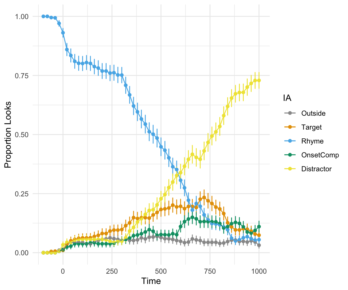
plot_avg(data = FinalDat, type = "proportion", xlim = c(-100, 1000), IAColumns = c(IA_Target_P = "Target", IA_Rhyme_P = "Rhyme", IA_OnsetComp_P = "OnsetComp", IA_Distractor_P = "Distractor"),Condition1 = NULL, Condition2 = NULL, Cond1Labels = NA, Cond2Labels = NA, ErrorBar = TRUE, VWPreTheme = FALSE) + theme_minimal() + scale_color_manual(values = cbPalette, labels = c("Target", "Rhyme", "OnsetComp", "Distractor"))## Grand average calculated using Event means.
## Scale for 'colour' is already present. Adding another scale for 'colour',
## which will replace the existing scale.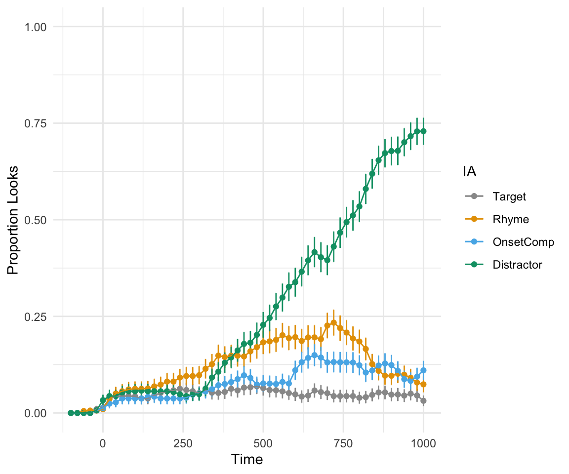
FinalDat2 = mutate(FinalDat, IA_234_P = IA_Rhyme_P + IA_OnsetComp_P + IA_Distractor_P)
plot_avg(data = FinalDat2, type = "proportion", xlim = c(-100, 1000), IAColumns = c(IA_Target_P = "Target", IA_234_P = "Non-Targets"),Condition1 = NULL, Condition2 = NULL, Cond1Labels = NA, Cond2Labels = NA, ErrorBar = TRUE, VWPreTheme = FALSE) + theme_minimal() + scale_color_manual(values = cbPalette, labels = c("Target", "Non-Target"))
## Grand average calculated using Event means.
## Scale for 'colour' is already present. Adding another scale for 'colour',
## which will replace the existing scale.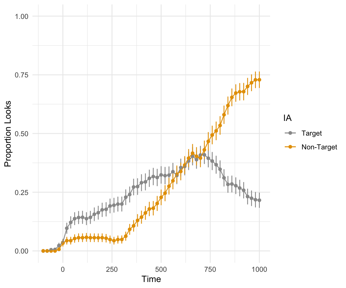
eyetrackingR
In eyetrackingR, the data is given to the plot() function, which passes into the plot.time_sequence_data() function. This is also built based on ggplot2 syntax.
However, one downfall of this function is that it automatically facets based on the predictor column given. (This is useful if you have two or more types of target and your IAs in the visual world paradigm do not change. For example, you have animate vs. inanimate targets, and you are comparing looks to inanimate images vs. animate images vs, distractors, the proportion of looks will depend on whether the target image is inanimate or animate.)
You can recreate the plot on your own without faceting, however, using ggplot2. Here, I do so both with the outside looks included and excluded.
plot(etRdata3, predictor_column=NULL) + theme_minimal() +coord_cartesian(ylim = c(0,1), xlim = c(-100,1200)) ## Warning: `fun.y` is deprecated. Use `fun` instead.
ggplot(etRdata3, aes(x= Time, y = Prop, color = AOI)) + geom_smooth() + theme_minimal() + scale_color_manual(values = cbPalette) + ylab("Proportion of looks")## `geom_smooth()` using method = 'gam' and formula 'y ~ s(x, bs = "cs")'## Warning: Computation failed in `stat_smooth()`:
## NA/NaN/Inf in foreign function call (arg 3)
ggplot(etRdata3, aes(x= Time, y = Prop, color = AOI)) + stat_summary(geom = "point", fun.y = "mean") + stat_summary(geom = "line", fun.y = "mean") + stat_summary(fun.data = mean_se , geom = "errorbar", width = 0)+ theme_minimal() + scale_color_manual(values = cbPalette)+ ylab("Proportion of looks")## Warning: `fun.y` is deprecated. Use `fun` instead.
## Warning: `fun.y` is deprecated. Use `fun` instead.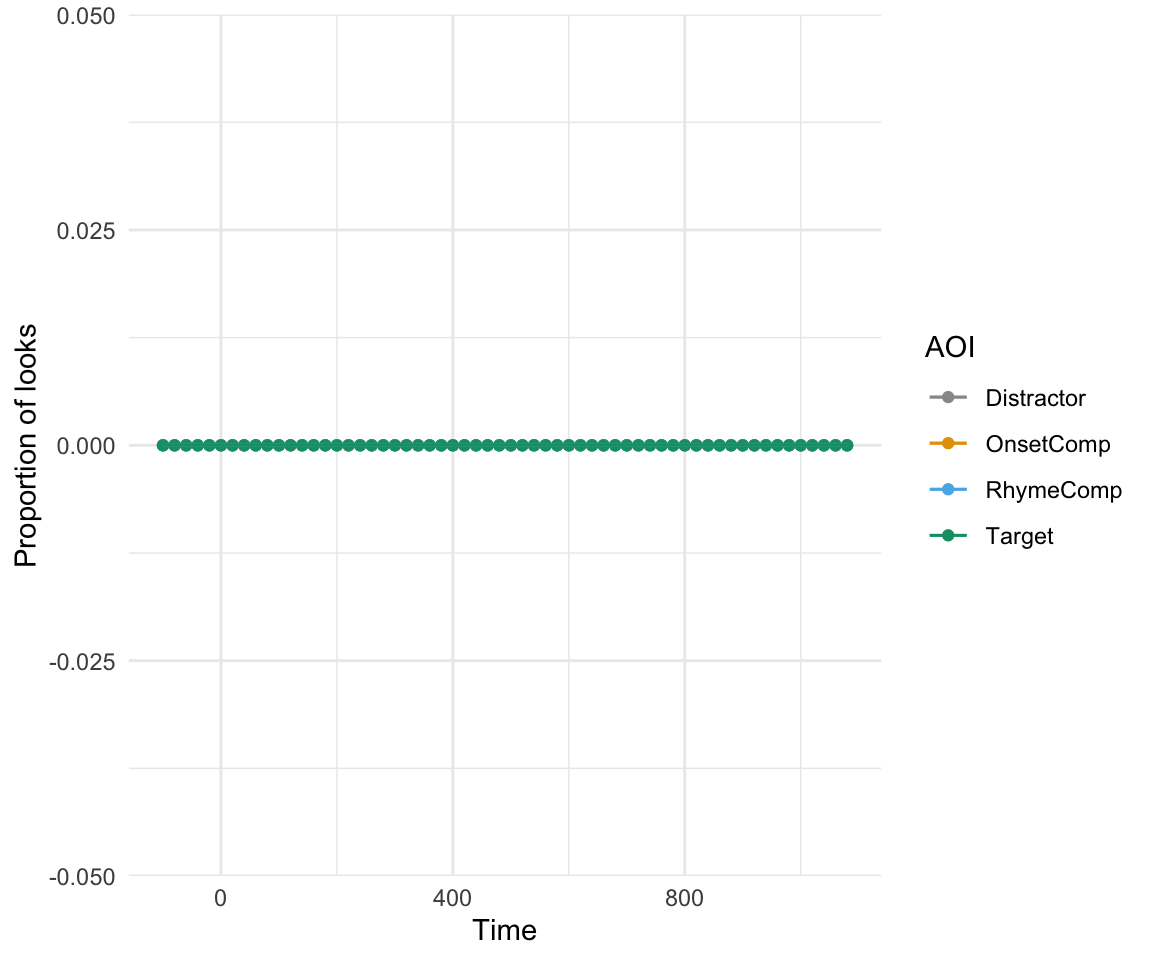
ggplot(etRdata3a, aes(x= Time, y = Prop, color = AOI)) + geom_smooth() + theme_minimal() + scale_color_manual(values = cbPalette)+ ylab("Proportion of looks")## `geom_smooth()` using method = 'gam' and formula 'y ~ s(x, bs = "cs")'## Warning: Computation failed in `stat_smooth()`:
## NA/NaN/Inf in foreign function call (arg 3)
ggplot(etRdata3a, aes(x= Time, y = Prop, color = AOI)) + stat_summary(geom = "point", fun.y = "mean") + stat_summary(geom = "line", fun.y = "mean") + stat_summary(fun.data = mean_se , geom = "errorbar", width = 0)+ theme_minimal() + scale_color_manual(values = cbPalette)+ ylab("Proportion of looks")+coord_cartesian(ylim = c(0,1), xlim = c(-100,1200)) ## Warning: `fun.y` is deprecated. Use `fun` instead.
## Warning: `fun.y` is deprecated. Use `fun` instead.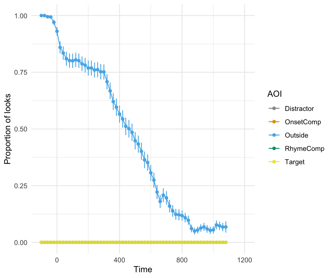
Note the difference if we had set treat_non_aoi_looks_as_missing to TRUE:
etRdatab <- make_eyetrackingr_data(VWdat2,
                               participant_column = "RECORDING_SESSION_LABEL",
                               trial_column = "TRIAL_INDEX",
                               time_column = "TIMESTAMP",
                               aoi_columns = c("Target","OnsetComp", "RhymeComp", "Distractor"),
                               treat_non_aoi_looks_as_missing = TRUE, trackloss_column = "TrackLoss")
## Converting Participants to proper type.## Converting Trial to proper type.etRdata2b <- subset_by_window(etRdatab, window_start_msg = "TargetOnset", msg_col = "SAMPLE_MESSAGE", rezero= TRUE, remove = FALSE)
etRdata3b = make_time_sequence_data(etRdata2b, time_bin_size = 20, predictor_columns = c("talker", "Exp"), aois = c("Target","OnsetComp", "RhymeComp", "Distractor")) %>% arrange(RECORDING_SESSION_LABEL, TRIAL_INDEX)## Analyzing Target...## Analyzing OnsetComp...## Analyzing RhymeComp...## Analyzing Distractor...ggplot(etRdata3b, aes(x= Time, y = Prop, color = AOI)) + stat_summary(geom = "point", fun.y = "mean") + stat_summary(geom = "line", fun.y = "mean") + stat_summary(fun.data = mean_se , geom = "errorbar", width = 0)+ theme_minimal() + scale_color_manual(values = cbPalette)+ ylab("Proportion of looks") +coord_cartesian(ylim = c(0,1), xlim = c(-100,1200)) 
Data analysis
There are a few different methods I have seen in the literature regarding how to analyze this data. I will go through a few of them here. Note that while the VWPre package is aimed at doing preprocessing of data, the eyetrackingR package has built in capabilities for running these analyses, so I will be showing you how to run the first two analyses using this package.
Linear mixed effects regression
Linear mixed effects regression (LMER) is a commonly-used methodology for doing eye-tracking analysis. However, with LMER, time has to be removed as a factor. In this case, looks within a specific window are generally averaged. (This is the method used in Ryskin et al., 2016).
The eyetrackingR package has a function, make_time_window_data(), which collapses time across a window and returns the data frame for LMER analysis. This should be used on the subsetted data, which we will create using subset_by_window(). Here, I am splitting the data into 3 windows of 400 ms each.
etRdata4a <- subset_by_window(etRdata2, window_start_time = 0, window_end_time = 400, rezero= FALSE, remove =TRUE)## Avg. window length in new data will be 400etRdata4b <- subset_by_window(etRdata2, window_start_time = 400, window_end_time = 800, rezero= FALSE, remove =TRUE)## Avg. window length in new data will be 400etRdata4c <- subset_by_window(etRdata2, window_start_time = 800, window_end_time = 1200, rezero= FALSE, remove =TRUE)## Avg. window length in new data will be 400etRdata5a = make_time_window_data(etRdata4a, aois = c("Target","OnsetComp", "RhymeComp", "Distractor"), predictor_columns = c("talker","Exp"))## Analyzing Target...## Analyzing OnsetComp...## Analyzing RhymeComp...## Analyzing Distractor...etRdata5b = make_time_window_data(etRdata4b, aois = c("Target","OnsetComp", "RhymeComp", "Distractor"), predictor_columns = c("talker","Exp"))## Analyzing Target...## Analyzing OnsetComp...## Analyzing RhymeComp...## Analyzing Distractor...etRdata5c = make_time_window_data(etRdata4c, aois = c("Target","OnsetComp", "RhymeComp", "Distractor"), predictor_columns = c("talker","Exp"))## Analyzing Target...## Analyzing OnsetComp...## Analyzing RhymeComp...## Analyzing Distractor...head(etRdata5a)## RECORDING_SESSION_LABEL TRIAL_INDEX talker Exp SamplesInAOI SamplesTotal
## 1 14001 1 EN3 High 0 400
## 2 14001 3 EN3 High 0 400
## 3 14001 8 EN3 High 0 400
## 4 14001 9 EN3 High 0 400
## 5 14001 10 EN3 High 0 400
## 6 14001 12 CH9 High 0 400
## AOI Elog Weights Prop LogitAdjusted ArcSin
## 1 Target -6.685861 0.001248439 0 NA 0
## 2 Target -6.685861 0.001248439 0 NA 0
## 3 Target -6.685861 0.001248439 0 NA 0
## 4 Target -6.685861 0.001248439 0 NA 0
## 5 Target -6.685861 0.001248439 0 NA 0
## 6 Target -6.685861 0.001248439 0 NA 0head(etRdata5b)## RECORDING_SESSION_LABEL TRIAL_INDEX talker Exp SamplesInAOI SamplesTotal
## 1 14001 1 EN3 High 0 400
## 2 14001 3 EN3 High 0 400
## 3 14001 8 EN3 High 0 400
## 4 14001 9 EN3 High 0 400
## 5 14001 10 EN3 High 0 400
## 6 14001 12 CH9 High 0 400
## AOI Elog Weights Prop LogitAdjusted ArcSin
## 1 Target -6.685861 0.001248439 0 NA 0
## 2 Target -6.685861 0.001248439 0 NA 0
## 3 Target -6.685861 0.001248439 0 NA 0
## 4 Target -6.685861 0.001248439 0 NA 0
## 5 Target -6.685861 0.001248439 0 NA 0
## 6 Target -6.685861 0.001248439 0 NA 0head(etRdata5c)## RECORDING_SESSION_LABEL TRIAL_INDEX talker Exp SamplesInAOI SamplesTotal
## 1 14001 1 EN3 High 0 281
## 2 14001 3 EN3 High 0 281
## 3 14001 8 EN3 High 0 281
## 4 14001 9 EN3 High 0 281
## 5 14001 10 EN3 High 0 280
## 6 14001 12 CH9 High 0 281
## AOI Elog Weights Prop LogitAdjusted ArcSin
## 1 Target -6.333280 0.001776199 0 NA 0
## 2 Target -6.333280 0.001776199 0 NA 0
## 3 Target -6.333280 0.001776199 0 NA 0
## 4 Target -6.333280 0.001776199 0 NA 0
## 5 Target -6.329721 0.001782531 0 NA 0
## 6 Target -6.333280 0.001776199 0 NA 0Now, we can run a linear model using lmer(). Here, I will see if the talker and listener experience has an influence on proportion of looks to the target word in each of the three time windows. There are 4 talkers (CH3, lowest proficiency in English, CH9 and CH10 (higher proficiency in English), and EN3, a native speaker) and 2 levels of listener experience (high, low).
library(lme4)
library(lmerTest)

etRlmera = lmer(Prop~talker*Exp + (1|RECORDING_SESSION_LABEL), data = subset(etRdata5a, AOI =="Target"))
summary(etRlmera)

etRlmerb = lmer(Prop~talker*Exp + (1|RECORDING_SESSION_LABEL), data = subset(etRdata5b, AOI =="Target"))
summary(etRlmerb)

etRlmerc = lmer(Prop~talker*Exp+ (1|RECORDING_SESSION_LABEL), data = subset(etRdata5c, AOI =="Target"))

summary(etRlmerc)
Growth curve analysis
Growth Curve Analysis (GCA) attempts to address the issue of taking time out of the equation by including it as an unaveraged predictor using polynomial functions. The eyetrackingR package actually includes these unaveraged polynomial predictors when it creates the time series data.
head(etRdata3)## # A tibble: 6 x 21
## RECORDING_SESSI… TRIAL_INDEX talker Exp TimeBin SamplesInAOI SamplesTotal
## <fct> <fct> <fct> <fct> <dbl> <int> <int>
## 1 14001 1 EN3 High -5 0 20
## 2 14001 1 EN3 High -4 0 20
## 3 14001 1 EN3 High -3 0 20
## 4 14001 1 EN3 High -2 0 20
## 5 14001 1 EN3 High -1 0 20
## 6 14001 1 EN3 High 0 0 20
## # … with 14 more variables: AOI <chr>, Elog <dbl>, Weights <dbl>, Prop <dbl>,
## # LogitAdjusted <lgl>, ArcSin <dbl>, Time <dbl>, ot1 <dbl>, ot2 <dbl>,
## # ot3 <dbl>, ot4 <dbl>, ot5 <dbl>, ot6 <dbl>, ot7 <dbl>timecodes <- unique(etRdata3[, c('ot1','ot2','ot3','ot4','ot5','ot6','ot7')])
timecodes$num <- 1:nrow(timecodes)
ggplot(timecodes, aes(x=num, y=ot1)) +
geom_line() +
geom_line(aes(y=ot2), color='red') + # quadratic
geom_line(aes(y=ot3), color='blue') + # cubic
geom_line(aes(y=ot4), color='green') + # quartic
geom_line(aes(y=ot5), color='purple') + # quintic
geom_line(aes(y=ot6), color='yellow') + # sextic
geom_line(aes(y=ot7), color='pink') + # septic
scale_x_continuous(name="") +
scale_y_continuous(name="") + theme_minimal()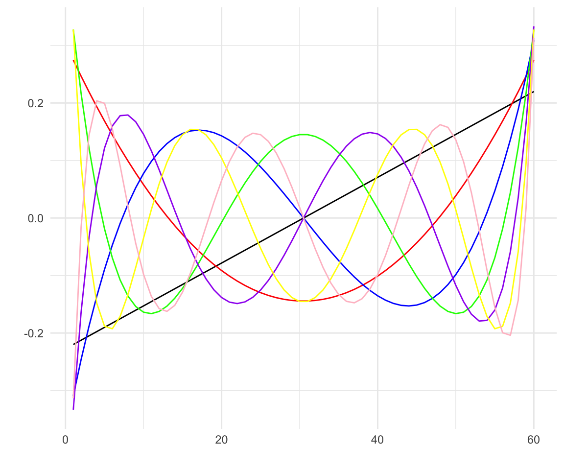
etRlmerGCA = lmer(Prop~talker*Exp*(ot1 + ot2 + ot3 + ot4)+ (1|RECORDING_SESSION_LABEL), data = subset(etRdata3, AOI =="Target"))
summary(etRlmerGCA)

plot(subset(etRdata3, AOI == "Target"), predictor_column = c("Exp"), model = etRlmerGCA) + theme_minimal()
plot(subset(etRdata3, AOI == "Target"), predictor_column = c("talker"), model = etRlmerGCA) + theme_minimal()
GCA can tell you that your conditions had some predictive value (i.e., changed differently) over time, and how those conditions changed by way of seeing which order polynomial has a significant effect on the model. However, they can’t tell you at what time these predictors had an effect. This is where GAM comes into play.
Generalized additive modeling
Generalized additive modeling (GAM) is a new nonlinear regression method, which relaxies the assumption of a linear relationship between predictors and predicted values. It has an advantage over growth curve analysis in that you can account for autocorrelation. I will not get into the nitty gritty details of GAM now, but I will show you the code for possible use of a GAM for this data.
library(mgcv)
library(itsadug)

etRdata3$AOI = as.factor(etRdata3$AOI)
etRdata3$Exp = as.factor(etRdata3$Exp)
etRdata3$talker = as.factor(etRdata3$talker)

etRgam = bam(Prop~talker*Exp + s(Time, by = AOI) + s(Time, by = Exp)+ s(Time, by = talker) + s(RECORDING_SESSION_LABEL, Time, by = AOI, bs = "fs", m=1), data = etRdata3)
summary(etRgam)

plot_smooth(etRgam, view = "Time", plot_all = "AOI", cond = list(talker = "CH1", Exp = "Low"))
plot_smooth(etRgam, view = "Time", plot_all = "AOI", cond = list(talker = "CH10", Exp = "High"))
plot_smooth(etRgam, view = "Time", plot_all = "AOI", cond = list(talker = "CH10", Exp = "Low"))
Conclusions and references
In short, there’s a lot you can do with eyetracking data. If you want to learn more about the eyetracking processing packages, here are some resources:
- VWPre: (https://cran.r-project.org/web/packages/VWPre/index.html)[https://cran.r-project.org/web/packages/VWPre/index.html] (go to the vignettes)
- eyetrackingR: (http://www.eyetracking-r.com/)[http://www.eyetracking-r.com/]
- GAM: (Wieling 2018)[https://www.sciencedirect.com/science/article/pii/S0095447017301377] (this is an excellent tutorial on how to use GAM for linguistic research, focused on phonological research but easily extended to any other time-series data)
- GAM with eyetracking: (Porretta et al. 2017)[https://link.springer.com/chapter/10.1007/978-3-319-59424-8_25#Sec2] (this is a proceedings chapter by the authors of the VWPre package, introducing how to use VWP data in a GAM setting)
- GAM with eyetracking: (Porretta et al. 2016)[https://www.sciencedirect.com/science/article/pii/S0095447016300146] (this is the paper the VWPre example data comes from, and it utilizes GAM for eyetracking in more detail. There is a lot of overlap between this paper and the previous proceedings paper.)