ERP Data Analysis in R
Preprocessing
Required packages
library(tidyverse)## ── Attaching packages ───────────────────────────────────────────────────────────────────────────────── tidyverse 1.3.0 ──## ✓ ggplot2 3.3.2 ✓ purrr 0.3.4
## ✓ tibble 3.0.3 ✓ dplyr 1.0.2
## ✓ tidyr 1.1.2 ✓ stringr 1.4.0
## ✓ readr 1.3.1 ✓ forcats 0.5.0## ── Conflicts ──────────────────────────────────────────────────────────────────────────────────── tidyverse_conflicts() ──
## x dplyr::filter() masks stats::filter()
## x dplyr::lag() masks stats::lag()library(mgcv)## Loading required package: nlme##
## Attaching package: 'nlme'## The following object is masked from 'package:dplyr':
##
## collapse## This is mgcv 1.8-31. For overview type 'help("mgcv-package")'.library(itsadug)## Loading required package: plotfunctions##
## Attaching package: 'plotfunctions'## The following object is masked from 'package:ggplot2':
##
## alpha## Loaded package itsadug 2.4 (see 'help("itsadug")' ).library(eegUtils)## Make sure to check for the latest development version at https://github.com/craddm/eegUtils!##
## Attaching package: 'eegUtils'## The following object is masked from 'package:stats':
##
## filter#devtools::install_github("craddm/eegUtils")
library(gridExtra)##
## Attaching package: 'gridExtra'## The following object is masked from 'package:dplyr':
##
## combinecbPalette <- c("#999999", "#E69F00", "#56B4E9", "#009E73", "#F0E442", "#0072B2", "#D55E00", "#CC79A7")Read in data
This data was kindly provided by Prof. Green.
The easiest way to read in data is to add each participant file to a list and then bind it all together. Often you have to initialize the ‘participant’ column yourself, possibly by taking that information out of the file name. Here since the participant code is a number, I use a regex to extract it from the filenames.
datadir = "/Users/marissabarlaz/Desktop/twix_results/"
mydata = list.files(path = datadir, pattern = "twix_.*")
mydata
## [1] "twix_0101.csv" "twix_0102.csv" "twix_0103.csv" "twix_0104.csv"
## [5] "twix_0105.csv" "twix_0106.csv" "twix_0107.csv"alldata = list()
for (k in 1:length(mydata)){
current_data = read_csv(paste0(datadir, mydata[k])) %>% mutate(Participant = str_extract(mydata[k], "[[:digit:]]+")) %>% select(Participant, everything())
alldata[[k]] = current_data
}## Parsed with column specification:
## cols(
## .default = col_double(),
## condition = col_character()
## )## See spec(...) for full column specifications.## Parsed with column specification:
## cols(
## .default = col_double(),
## condition = col_character()
## )## See spec(...) for full column specifications.## Parsed with column specification:
## cols(
## .default = col_double(),
## condition = col_character()
## )## See spec(...) for full column specifications.## Parsed with column specification:
## cols(
## .default = col_double(),
## condition = col_character()
## )## See spec(...) for full column specifications.## Parsed with column specification:
## cols(
## .default = col_double(),
## condition = col_character()
## )## See spec(...) for full column specifications.## Parsed with column specification:
## cols(
## .default = col_double(),
## condition = col_character()
## )## See spec(...) for full column specifications.## Parsed with column specification:
## cols(
## .default = col_double(),
## condition = col_character()
## )## See spec(...) for full column specifications.twix_data = do.call( "rbind", alldata) %>% mutate_at(.vars = c(1,2), .funs = as.factor)
head(twix_data)## # A tibble: 6 x 36
## Participant condition epoch time FP1 FP2 F7 F3 Fz F4 F8
## <fct> <fct> <dbl> <dbl> <dbl> <dbl> <dbl> <dbl> <dbl> <dbl> <dbl>
## 1 0101 S115 0 -200 30.5 32.7 18.6 11.5 12.8 7.25 6.15
## 2 0101 S115 0 -199 28.8 32.1 17.4 11.5 12.0 6.45 5.22
## 3 0101 S115 0 -198 27.0 31.4 16.2 11.7 11.3 5.80 4.40
## 4 0101 S115 0 -197 25.2 30.5 14.7 11.8 10.6 5.29 3.70
## 5 0101 S115 0 -196 23.5 29.5 13.2 12.1 9.92 4.93 3.15
## 6 0101 S115 0 -195 21.8 28.3 11.5 12.4 9.32 4.73 2.74
## # … with 25 more variables: FC5 <dbl>, FC1 <dbl>, FC2 <dbl>, FC6 <dbl>,
## # T7 <dbl>, C3 <dbl>, Cz <dbl>, C4 <dbl>, T8 <dbl>, CP5 <dbl>, CP1 <dbl>,
## # CP2 <dbl>, CP6 <dbl>, P7 <dbl>, P3 <dbl>, Pz <dbl>, P4 <dbl>, P8 <dbl>,
## # O1 <dbl>, Oz <dbl>, O2 <dbl>, LO1 <dbl>, LO2 <dbl>, IO1 <dbl>, M2 <dbl>dim(twix_data)## [1] 819819 36unique(twix_data$epoch)## [1] 0 1 2 3 4 5 6 7 8 9 10 11 12 13 14 15 16 17
## [19] 18 19 20 21 22 23 24 25 26 27 28 29 30 31 32 33 34 35
## [37] 36 37 38 39 40 41 42 43 44 45 46 47 48 49 50 51 52 53
## [55] 54 55 56 57 58 59 60 61 62 63 64 65 66 67 68 69 70 71
## [73] 72 73 74 75 76 77 78 79 80 81 82 83 84 85 86 87 88 89
## [91] 90 91 92 93 94 95 96 97 98 99 100 101 102 103 104 105 106 107
## [109] 108 109 110 111 112 113 114 115 116 117 118 119unique(twix_data$condition)## [1] S115 S125 S135
## Levels: S115 S125 S135Here I am reading in two different datasets - hemisphereinfo has anteriority and hemisphere, and electrodes has X and Y coordinates of the electrodes.
hemisphereinfo = read_csv("/Users/marissabarlaz/Desktop/twix_results/electrode_quadrants.csv")## Parsed with column specification:
## cols(
## Electrode = col_character(),
## Anteriority = col_character(),
## Hemisphere = col_character()
## )electrodes <- itsadug::eeg[,c('X','Y','Electrode')]
electrodes <- ( electrodes[!duplicated(electrodes),] )
electrodes$Electrode = toupper( electrodes$Electrode)Convert to long format, combine data frames
A previous function to make data long is gather(), however, this function is being retired in the tidyverse.
twix_data_long = twix_data %>% pivot_longer(-c(Participant:time), names_to= "Electrode", values_to = "uV") %>% left_join(hemisphereinfo, by = "Electrode") %>% left_join(electrodes, by = "Electrode") %>% select(Participant, condition, epoch, Anteriority, Hemisphere,Electrode, X, Y, time, uV)Plotting time courses
Note that many functions from the eegUtils package require the columns to have specific names.
Here I am plotting one participant’s data.
twix0101 = twix_data_long %>% filter(Participant == "0101")

twix0101 %>% filter(!is.na(Anteriority)) %>% ggplot(aes(x = time, y = uV)) +  stat_summary(fun.y = mean,geom = "line",aes(colour = condition)) + facet_grid(Hemisphere~Anteriority) + theme_minimal() + scale_color_manual(values = cbPalette)
## Warning: `fun.y` is deprecated. Use `fun` instead.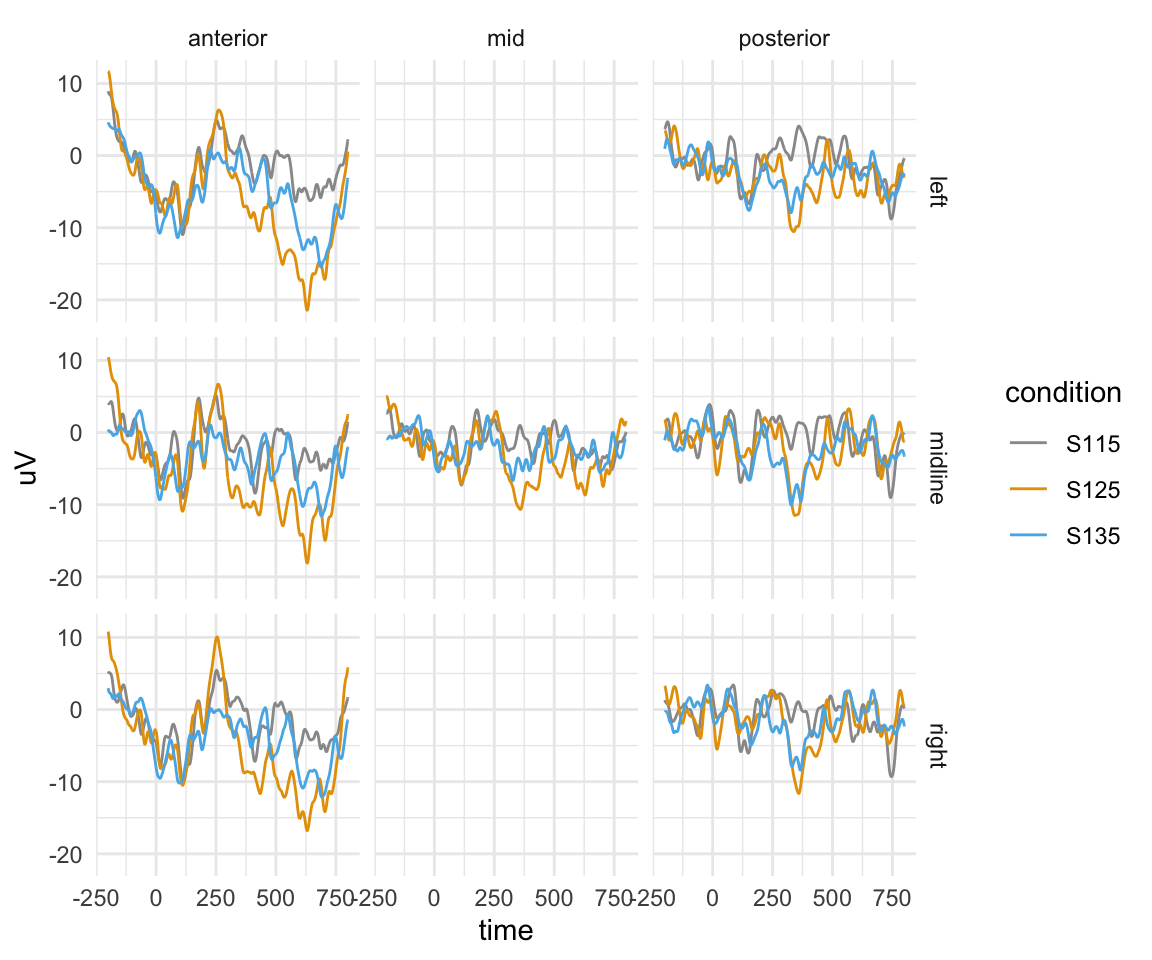
twix0101 %>% rename(electrode = Electrode, amplitude = uV) %>% plot_butterfly()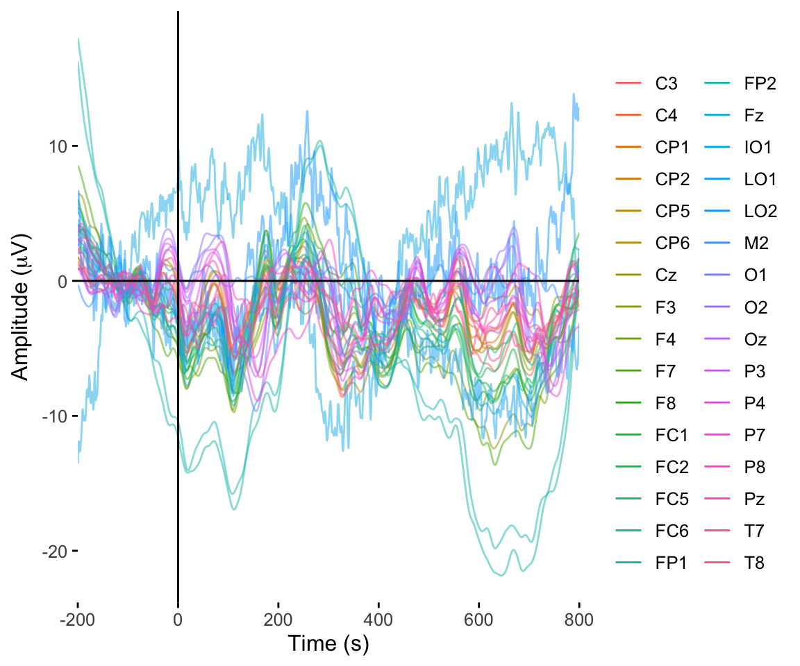
P600 and N400 calculations
Here I am creating two dataframes - one for P600, one for N400, and combining them.
twix_data_N400 = twix_data_long %>% filter(time <=500 & time >=300) %>% group_by(Participant, Hemisphere, Anteriority, condition) %>% summarise(N400 = mean(uV, na.rm = TRUE))## `summarise()` regrouping output by 'Participant', 'Hemisphere', 'Anteriority' (override with `.groups` argument)twix_data_P600 = twix_data_long %>% filter(time >=500 & time <=800) %>% group_by(Participant, Hemisphere, Anteriority, condition) %>% summarise(P600 = mean(uV, na.rm = TRUE))## `summarise()` regrouping output by 'Participant', 'Hemisphere', 'Anteriority' (override with `.groups` argument)twix_effects = full_join(twix_data_N400, twix_data_P600)## Joining, by = c("Participant", "Hemisphere", "Anteriority", "condition")ANOVA
summary(aov(N400~condition*Hemisphere, data = filter(twix_effects, Hemisphere!="midline", Anteriority=="posterior")))## Df Sum Sq Mean Sq F value Pr(>F)
## condition 2 154.79 77.39 35.860 2.7e-09 ***
## Hemisphere 1 1.46 1.46 0.678 0.416
## condition:Hemisphere 2 0.52 0.26 0.121 0.887
## Residuals 36 77.70 2.16
## ---
## Signif. codes: 0 '***' 0.001 '**' 0.01 '*' 0.05 '.' 0.1 ' ' 1summary(aov(P600~Anteriority*condition*Hemisphere, data = twix_effects))## Df Sum Sq Mean Sq F value Pr(>F)
## Anteriority 2 166.1 83.04 10.000 9.31e-05 ***
## condition 2 17.1 8.54 1.028 0.3606
## Hemisphere 2 18.8 9.40 1.132 0.3255
## Anteriority:condition 4 67.3 16.82 2.025 0.0948 .
## Anteriority:Hemisphere 2 0.3 0.15 0.018 0.9820
## condition:Hemisphere 4 5.8 1.44 0.173 0.9517
## Anteriority:condition:Hemisphere 4 1.2 0.30 0.036 0.9975
## Residuals 126 1046.2 8.30
## ---
## Signif. codes: 0 '***' 0.001 '**' 0.01 '*' 0.05 '.' 0.1 ' ' 1
## 21 observations deleted due to missingnessk means clustering
Darren Tanner used k-means clustering in this paper. His use of k-means clustering was an exploratory analysis. He used this method to compare two test conditions to baseline.
Here I am comparing conditions S125 and S135 each to baseline S115. The first steps are creating the data frames.
twix_data_N400_diff = twix_data_N400 %>% ungroup() %>% pivot_wider( names_from = condition, values_from = N400) %>% mutate(N400_S2_1 = S125-S115, N400_S3_1 = S135-S115) %>% select(-c(S115:S135))


twix_data_P600_diff = twix_data_P600 %>% ungroup() %>% pivot_wider( names_from = condition, values_from = P600) %>% mutate(P600_S2_1 = S125-S115, P600_S3_1 = S135-S115) %>% select(-c(S115:S135))

head(twix_data_P600_diff)
## # A tibble: 6 x 5
## Participant Hemisphere Anteriority P600_S2_1 P600_S3_1
## <fct> <chr> <chr> <dbl> <dbl>
## 1 0101 left anterior -10.3 -6.29
## 2 0101 left posterior -1.22 -0.255
## 3 0101 midline anterior -7.48 -3.42
## 4 0101 midline mid -2.06 -0.154
## 5 0101 midline posterior 0.486 0.422
## 6 0101 right anterior -7.43 -4.03twix_diff = full_join(twix_data_N400_diff, twix_data_P600_diff) %>% filter(!is.na(Hemisphere)) %>% pivot_wider(id_cols = Participant, names_from = c(Anteriority, Hemisphere), values_from = c(N400_S2_1:P600_S3_1))## Joining, by = c("Participant", "Hemisphere", "Anteriority")head(twix_diff)## # A tibble: 6 x 29
## Participant N400_S2_1_anter… N400_S2_1_poste… N400_S2_1_anter…
## <fct> <dbl> <dbl> <dbl>
## 1 0101 -6.27 -6.75 -5.57
## 2 0102 -2.62 -3.93 -1.56
## 3 0103 -7.60 -3.41 -9.61
## 4 0104 -2.41 -2.91 -2.10
## 5 0105 0.696 -3.22 0.429
## 6 0106 -2.51 -2.52 -4.89
## # … with 25 more variables: N400_S2_1_mid_midline <dbl>,
## # N400_S2_1_posterior_midline <dbl>, N400_S2_1_anterior_right <dbl>,
## # N400_S2_1_posterior_right <dbl>, N400_S3_1_anterior_left <dbl>,
## # N400_S3_1_posterior_left <dbl>, N400_S3_1_anterior_midline <dbl>,
## # N400_S3_1_mid_midline <dbl>, N400_S3_1_posterior_midline <dbl>,
## # N400_S3_1_anterior_right <dbl>, N400_S3_1_posterior_right <dbl>,
## # P600_S2_1_anterior_left <dbl>, P600_S2_1_posterior_left <dbl>,
## # P600_S2_1_anterior_midline <dbl>, P600_S2_1_mid_midline <dbl>,
## # P600_S2_1_posterior_midline <dbl>, P600_S2_1_anterior_right <dbl>,
## # P600_S2_1_posterior_right <dbl>, P600_S3_1_anterior_left <dbl>,
## # P600_S3_1_posterior_left <dbl>, P600_S3_1_anterior_midline <dbl>,
## # P600_S3_1_mid_midline <dbl>, P600_S3_1_posterior_midline <dbl>,
## # P600_S3_1_anterior_right <dbl>, P600_S3_1_posterior_right <dbl>Here I am running k-means clustering by giving the function the columns for each condition. I am specifying 2 groups (i.e., centers). I am then adding this information to the wide dataframe.
twix_kmeans_2_1 = kmeans(twix_diff[,c(2:8,16:22)], centers = 2)

twix_kmeans_3_1 = kmeans(twix_diff[,c(9:15,23:29)], centers = 2)

twix_diff$cluster2_1 = twix_kmeans_2_1$cluster

twix_diff$cluster3_1 = twix_kmeans_3_1$cluster

twix_diff = twix_diff %>% select(Participant, cluster2_1, cluster3_1, everything())
Plotting
Note that the topoplot() function (from eegUtils) requires specific column names, hence the rename function.
I am plotting a single person from each cluster, for each of these condition comparisons. To plot four figures in one plot, I am using the grid.arrange() function from the gridExtra package.
S125 - S115
n400s1251 = twix_data_long %>% filter(Participant =="0101", condition == "S125") %>% rename(electrode = Electrode, x = X, y = Y, amplitude = uV) %>% topoplot(time_lim = c(300,500)) + ggtitle("N400, cluster 1, condition S125")## Using electrode locations from data.## Warning in topoplot.data.frame(., time_lim = c(300, 500)): Removing channels
## with no location.p600s1251 = twix_data_long %>% filter(Participant =="0101", condition == "S125") %>% rename(electrode = Electrode, x = X, y = Y, amplitude = uV) %>% topoplot(time_lim = c(500,800)) + ggtitle("P600, cluster 1, condition S125")## Using electrode locations from data.## Warning in topoplot.data.frame(., time_lim = c(500, 800)): Removing channels
## with no location.n400s1252 = twix_data_long %>% filter(Participant =="0102", condition == "S125") %>% rename(electrode = Electrode, x = X, y = Y, amplitude = uV) %>% topoplot(time_lim = c(300,500)) + ggtitle("N400, cluster 2, condition S125")## Using electrode locations from data.## Warning in topoplot.data.frame(., time_lim = c(300, 500)): Removing channels
## with no location.p600s1252 = twix_data_long %>% filter(Participant =="0102", condition == "S125") %>% rename(electrode = Electrode, x = X, y = Y, amplitude = uV) %>% topoplot(time_lim = c(500,800)) +ggtitle("P600, cluster 2, condition S125")## Using electrode locations from data.## Warning in topoplot.data.frame(., time_lim = c(500, 800)): Removing channels
## with no location.grid.arrange(n400s1251, p600s1251, n400s1252, p600s1252, nrow = 2)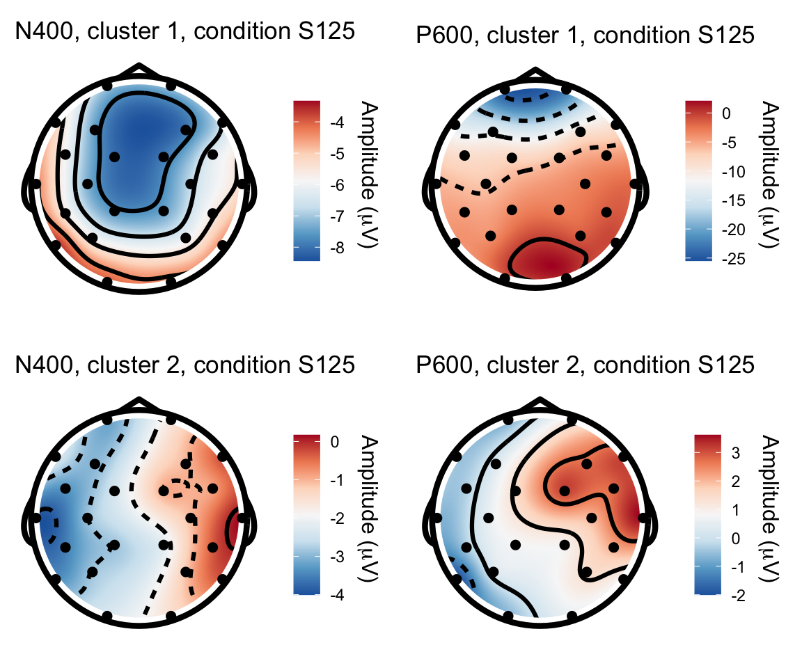
S135 - S115
n400s1351 = twix_data_long %>% filter(Participant =="0107", condition == "S135") %>% rename(electrode = Electrode, x = X, y = Y, amplitude = uV) %>% topoplot(time_lim = c(300,500)) + ggtitle("N400, cluster 1, condition S135")## Using electrode locations from data.## Warning in topoplot.data.frame(., time_lim = c(300, 500)): Removing channels
## with no location.p600s1351 = twix_data_long %>% filter(Participant =="0107", condition == "S135") %>% rename(electrode = Electrode, x = X, y = Y, amplitude = uV) %>% topoplot(time_lim = c(500,800)) + ggtitle("P600, cluster 1, condition S135")## Using electrode locations from data.## Warning in topoplot.data.frame(., time_lim = c(500, 800)): Removing channels
## with no location.n400s1352 = twix_data_long %>% filter(Participant =="0102", condition == "S135") %>% rename(electrode = Electrode, x = X, y = Y, amplitude = uV) %>% topoplot(time_lim = c(300,500)) + ggtitle("N400, cluster 2, condition S135")## Using electrode locations from data.## Warning in topoplot.data.frame(., time_lim = c(300, 500)): Removing channels
## with no location.p600s1352 = twix_data_long %>% filter(Participant =="0102", condition == "S135") %>% rename(electrode = Electrode, x = X, y = Y, amplitude = uV) %>% topoplot(time_lim = c(500,800)) +ggtitle("P600, cluster 2, condition S135")## Using electrode locations from data.## Warning in topoplot.data.frame(., time_lim = c(500, 800)): Removing channels
## with no location.grid.arrange(n400s1351, p600s1351, n400s1352, p600s1352, nrow = 2)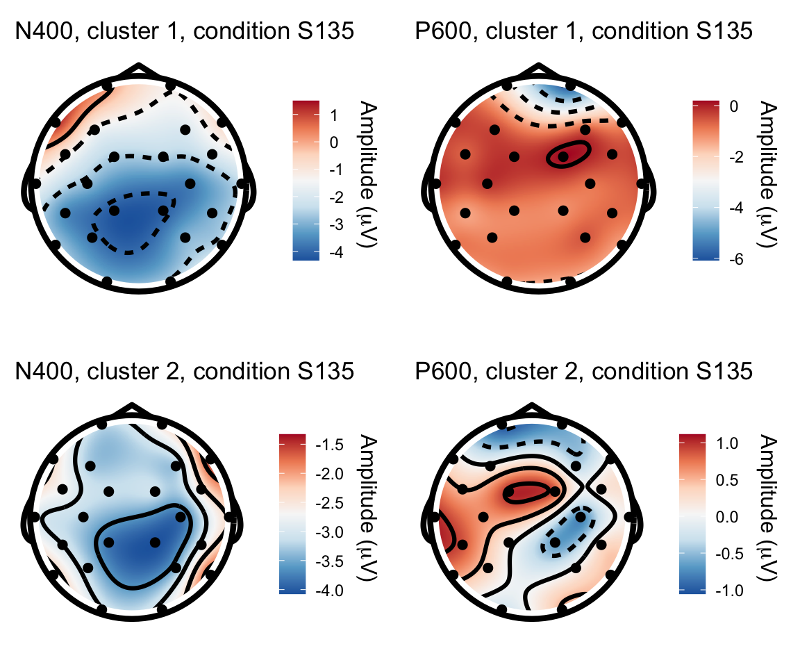
GAM
For computational purposes I am only looking at one participant. This model took me 15 minutes to run on my personal laptop.
twix0101 = twix_data_long %>% filter(Participant == "0101")

gamtwix0101 = bam(uV~te(time, X,Y, by = condition), data = twix0101)
summary(gamtwix0101)
##
## Family: gaussian
## Link function: identity
##
## Formula:
## uV ~ te(time, X, Y, by = condition)
##
## Parametric coefficients:
## Estimate Std. Error t value Pr(>|t|)
## (Intercept) -2.71382 0.01299 -209 <2e-16 ***
## ---
## Signif. codes: 0 '***' 0.001 '**' 0.01 '*' 0.05 '.' 0.1 ' ' 1
##
## Approximate significance of smooth terms:
## edf Ref.df F p-value
## te(time,X,Y):conditionS115 84.74 94.56 137.4 <2e-16 ***
## te(time,X,Y):conditionS125 88.42 97.51 554.5 <2e-16 ***
## te(time,X,Y):conditionS135 88.42 97.50 280.4 <2e-16 ***
## ---
## Signif. codes: 0 '***' 0.001 '**' 0.01 '*' 0.05 '.' 0.1 ' ' 1
##
## R-sq.(adj) = 0.0374 Deviance explained = 3.75%
## fREML = 1.0729e+07 Scale est. = 405.6 n = 2426424#not run:
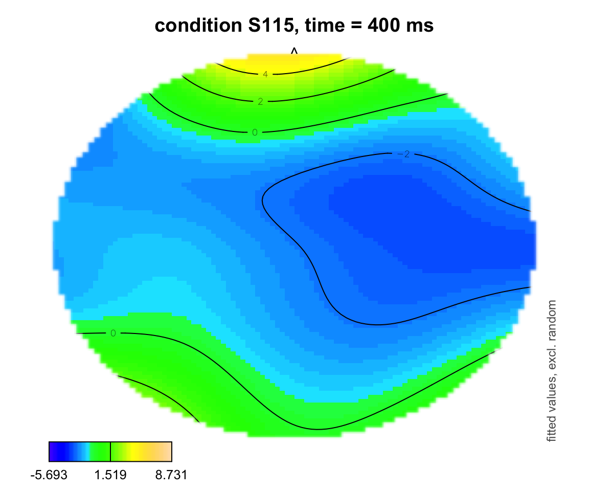
#gamtwixall = bam(uV~te(time, X,Y, by = condition) + s(time,X,Y, Participant, by = condition, bs = "fs", m =1), data = twix_data_long)topo plotting
plot_topo(gamtwix0101, view = c("X", "Y"), cond = list(time = 400, condition = "S115"), color = "topo", main = "condition S115, time = 400 ms")## Summary:
## * time : numeric predictor; set to the value(s): 400.
## * X : numeric predictor; with 100 values ranging from -46.200000 to 46.200000.
## * Y : numeric predictor; with 100 values ranging from -46.200000 to 46.200000.
## * condition : factor; set to the value(s): S115.
## * NOTE : No random effects in the model to cancel.
## 
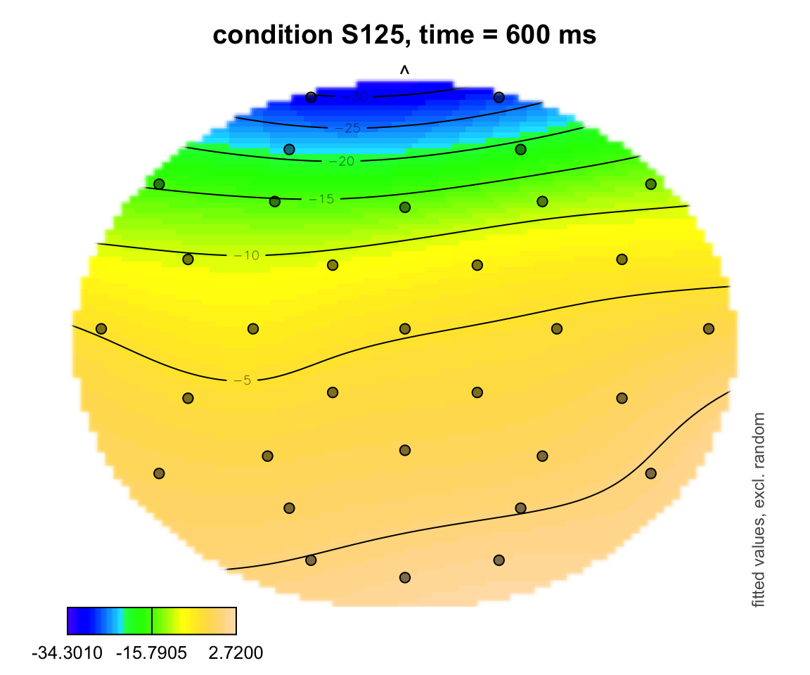
#Add electrode sites
plot_topo(gamtwix0101, view = c("X", "Y"), cond = list(time = 600, condition = "S125"), color = "topo", el.pos = electrodes,  main = "condition S125, time = 600 ms")
## Summary:
## * time : numeric predictor; set to the value(s): 600.
## * X : numeric predictor; with 100 values ranging from -46.200000 to 46.200000.
## * Y : numeric predictor; with 100 values ranging from -47.700000 to 44.700000.
## * condition : factor; set to the value(s): S125.
## * NOTE : No random effects in the model to cancel.
## 
# Add labels:
plot_topo(gamtwix0101, view=c('X', 'Y'), cond=list(time=200, condition = "S135"))
## Summary:
## * time : numeric predictor; set to the value(s): 200.
## * X : numeric predictor; with 100 values ranging from -46.200000 to 46.200000.
## * Y : numeric predictor; with 100 values ranging from -46.200000 to 46.200000.
## * condition : factor; set to the value(s): S135.
## * NOTE : No random effects in the model to cancel.
## text(electrodes[['X']], electrodes[['Y']],
labels=electrodes[['Electrode']], cex=.75,
xpd=TRUE)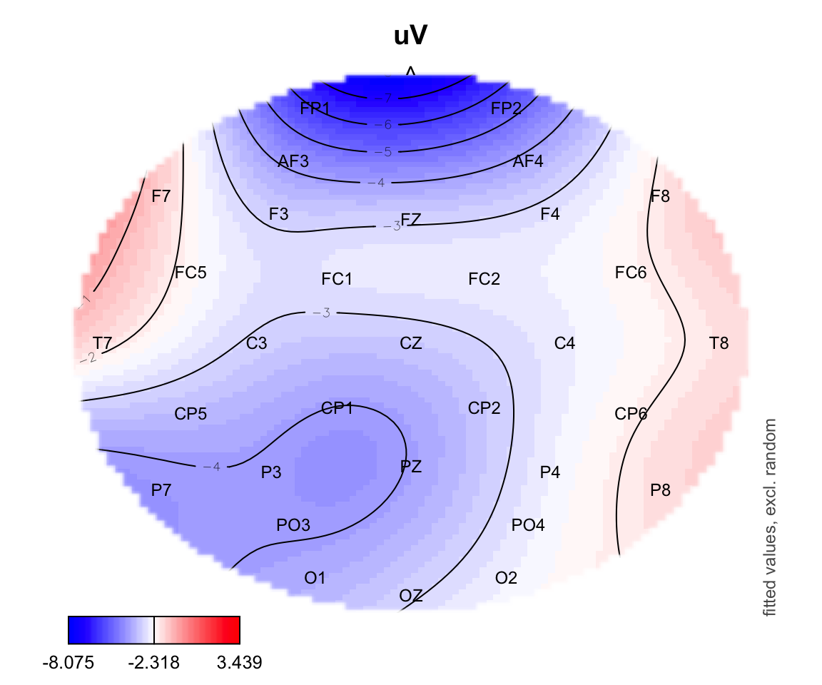
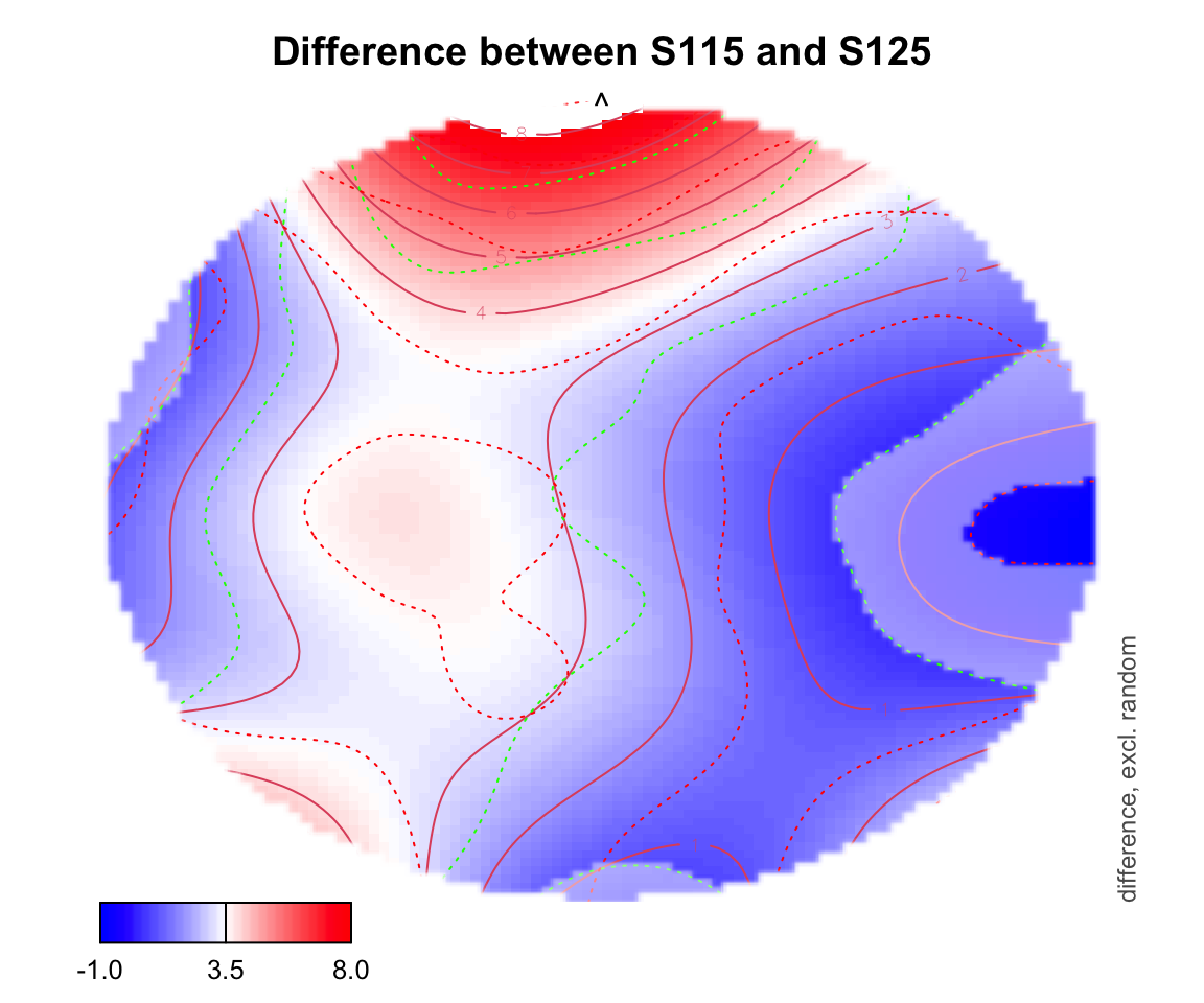
Difference plotting
For difference plotting, you need to specify a zlim in order to see the color bar on the bottom. zlim is the range of differences between two conditions. Figuring out an appropriate zlim takes some trial and error. If a value is outside of that zlim range, it shows up as white on the topo plot.
plot_topo(gamtwix0101, view=c('X', 'Y'), zlim = c(-1,8),
cond = list(time = 400), comp=list(condition = c("S115", "S125")),
fun='plot_diff2')## Summary:
## * time : numeric predictor; set to the value(s): 400.
## * X : numeric predictor; with 100 values ranging from -46.200000 to 46.200000.
## * Y : numeric predictor; with 100 values ranging from -46.200000 to 46.200000.
## * NOTE : No random effects in the model to cancel.
## 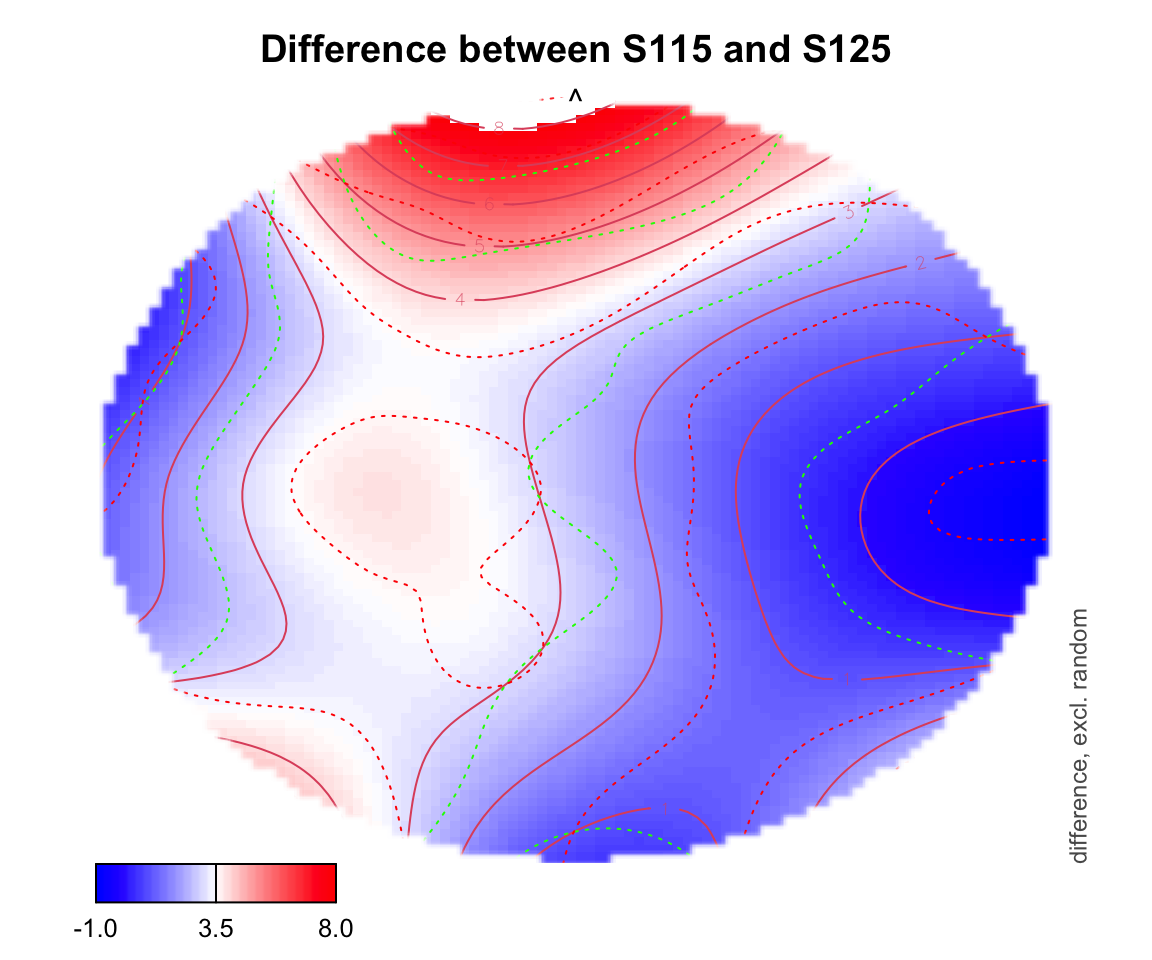
plot_topo(gamtwix0101, view=c('X', 'Y'), zlim = c(-1,8),
cond = list(time = 400), comp=list(condition = c("S115", "S125")),
fun='plot_diff2', show.diff = T, col.diff = "white")## Summary:
## * time : numeric predictor; set to the value(s): 400.
## * X : numeric predictor; with 100 values ranging from -46.200000 to 46.200000.
## * Y : numeric predictor; with 100 values ranging from -46.200000 to 46.200000.
## * NOTE : No random effects in the model to cancel.
## 
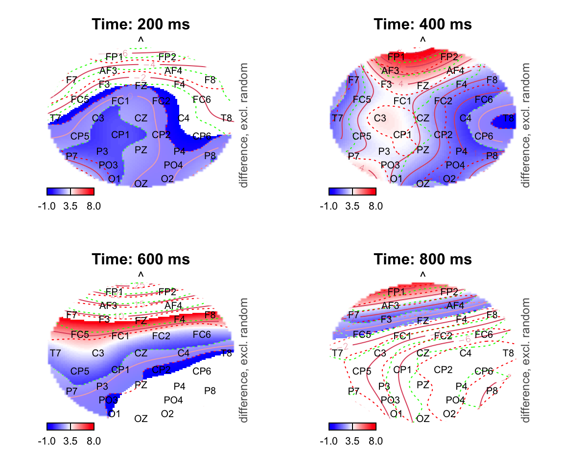
par(mfrow = c(2,2))
for (k in c(200,400,600,800)){
plot_topo(gamtwix0101, view=c('X', 'Y'), zlim = c(-1,8),
cond = list(time = k), comp=list(condition = c("S115", "S125")),
fun='plot_diff2', main = paste0("Time: ", k, " ms"), show.diff = T, col.diff = "white")
text(electrodes[['X']], electrodes[['Y']],
    labels=electrodes[['Electrode']], cex=.75,
    xpd=TRUE)
}## Summary:
## * time : numeric predictor; set to the value(s): 200.
## * X : numeric predictor; with 100 values ranging from -46.200000 to 46.200000.
## * Y : numeric predictor; with 100 values ranging from -46.200000 to 46.200000.
## * NOTE : No random effects in the model to cancel.
## ## Summary:
## * time : numeric predictor; set to the value(s): 400.
## * X : numeric predictor; with 100 values ranging from -46.200000 to 46.200000.
## * Y : numeric predictor; with 100 values ranging from -46.200000 to 46.200000.
## * NOTE : No random effects in the model to cancel.
## ## Summary:
## * time : numeric predictor; set to the value(s): 600.
## * X : numeric predictor; with 100 values ranging from -46.200000 to 46.200000.
## * Y : numeric predictor; with 100 values ranging from -46.200000 to 46.200000.
## * NOTE : No random effects in the model to cancel.
## ## Summary:
## * time : numeric predictor; set to the value(s): 800.
## * X : numeric predictor; with 100 values ranging from -46.200000 to 46.200000.
## * Y : numeric predictor; with 100 values ranging from -46.200000 to 46.200000.
## * NOTE : No random effects in the model to cancel.
## 
Making a movie
library(av)
for (k in seq(from = 0,to = 800,by = 20)){
  nameme = paste0("~/Desktop/twix_png/twix", sprintf("%03d", k), ".png")
  png(nameme)
  plot_topo(gamtwix0101, view=c('X', 'Y'), zlim = c(-8,8),
            cond = list(time = k), comp=list(condition = c("S125", "S115")),
            fun='plot_diff2', main = paste0("Time: ", k, " ms"), show.diff = T, col.diff = "white")
  dev.off()

}


png_files <- sprintf("~/Desktop/twix_png/twix%03d.png", seq(0,800,20))
av::av_encode_video(png_files, '~/Desktop/twix_png/output.mp4', framerate = 10)