Data Processing with the Tidyverse
#Why the tidyverse?
There are a few reasons to use R and the Tidyverse for data processing. Excel is opaque – if you make a change to a cell/row/column, unless you write down exactly what you did, you have no way of knowing how you processed your data. Using R and documenting your work in Rmarkdown will allow you to understand exactly what you are doing, which is helpful in future iterations of using the data.
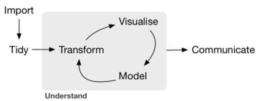
Chances are, you are not going to get data from an experiment in a form that is ready to go for an analysis.Therefore, it is important to first figure out what shape you want your data to be in before you start processing. That way, you have a clear way forward towards tidy data. Tidying and transforming are called ‘wrangling’, a term you will see often in the field of data science.
##Tidy data There are three interrelated rules which make a dataset tidy:
- Each variable must have its own column.
- Each observation must have its own row.
- Each value must have its own cell.
Data doesn’t often come in this form. For example, sometimes we have data spread over various files (e.g., a file for each speaker/participant). Other untidy datasets have multiple variables over multiple columns. For example, variable name is in one column, and then the value is in a second column. Using the tidyverse, we can take this untidy data and make it tidy!
##Components of the tidyverse require(tidyverse) installs the following packages (and some others):
- ggplot2: creates graphics
- dplyr: data manipulation
- tidyr: tidies data
- readr: allows you to read in rectangular data (fwf, csv, etc.)
- tibble: allows you to make tibbles and convert to and from data frames
- stringr: works with character strings
Other packages that are part of the tidyverse that you have to require individually: * readxl: imports excel files * magrittr: helps with programming, including different pipes * broom: formats models into tidy data * modelr: Helper functions for modeling data
##Importing data
Importing data is essential – if you can’t import your data, you can’t analyze it! Make sure to include any code relating to importing in your Rmarkdown document, so if you make a mistake you don’t have to go back to square one.
Use the read.table(), read.csv(), or read_excel() functions to import your data. Remember to name your data something descriptive, and not too long. If you want to totally emerse yourself in the tidyverse, you can use readr::read_csv() or readr::read_table(), which will import your data as a tibble.
##The pipe operator With base R, we run various data wrangling techniques on the dataset one at a time. In each of these cases, we would either overwrite the original dataset, or save the intermediate steps as new variables. This makes your workspace messy very quickly. The pipe operator (based in tidyverse package magrittr) allows multiple steps of data wrangling or analysis to occur in succession, without creating multiple intermediate dataframes. This works by dropping the input into the first argument space.
x %>% f is equivalent to f(x)
x %>% f(y) is equivalent to f(x, y)
x %>% f %>% g %>% h is equivalent to h(g(f(x)))
So, for example:
nasality %>% head() is equivalent to head(nasality)
nasality %>% str() is equivalent to str(nasality)
nasality %>% filter(freq_f3>2400) is equivalent to filter(nasality, freq_f3 > 2400)
However, this doesn’t work: nasality %>% sd(freq_f1)
If you wanted to put the left-hand-side object into a subsequent argument slot using the pipe, use the placeholder . to denote the location where you want the left-hand-side argument to go:
2 %>% round(nasality$F1, digits = .)This translates to round(nasality$F1, digits = 2)
Data Manipulation with dplyr
What dataset are we using? This is my dissertation data. I have processed this a bit, without showing you the code. I will show you the code I used to process it at the end.
The data is as follows: I have formant data (F1-3, and the difference between F2 and F3) at ten normalized time points, for various vowels. The vowel categories are /a/, /i/, and /u/, spoken by 12 Brazilian Portuguese speakers, in the following nasality conditions: oral, nasalized, and nasal (word-final and word-medial). Therefore, there are 12 (vowel*nasality) combinations for each speaker.
Note that in this file you will only see 20 rows of each tibble. This is on purpose, in order to make the file size smaller. The actual size of the data is on the order of 64k rows.
head(normtimedata)## # A tibble: 6 x 13
## Speaker Word Vowel Nasality RepNo NormTime Type label Time F1 F2
## <chr> <chr> <chr> <chr> <int> <dbl> <chr> <chr> <dbl> <dbl> <dbl>
## 1 BP02 abun… u nasal 1 0.1 clean un 3.39 569. 2372.
## 2 BP02 abun… u nasal 1 0.2 clean un 3.41 364. 2297.
## 3 BP02 abun… u nasal 1 0.3 clean un 3.43 373. 2258.
## 4 BP02 abun… u nasal 1 0.4 clean un 3.46 303. 2165.
## 5 BP02 abun… u nasal 1 0.5 clean un 3.48 415. 2247.
## 6 BP02 abun… u nasal 1 0.6 clean un 3.51 336. 2098.
## # … with 2 more variables: F3 <dbl>, F2_3 <dbl>str(normtimedata)## tibble [182,150 × 13] (S3: tbl_df/tbl/data.frame)
## $ Speaker : chr [1:182150] "BP02" "BP02" "BP02" "BP02" ...
## $ Word : chr [1:182150] "abunda" "abunda" "abunda" "abunda" ...
## $ Vowel : chr [1:182150] "u" "u" "u" "u" ...
## $ Nasality: chr [1:182150] "nasal" "nasal" "nasal" "nasal" ...
## $ RepNo : int [1:182150] 1 1 1 1 1 1 1 1 1 1 ...
## $ NormTime: num [1:182150] 0.1 0.2 0.3 0.4 0.5 0.6 0.7 0.8 0.9 1 ...
## $ Type : chr [1:182150] "clean" "clean" "clean" "clean" ...
## $ label : chr [1:182150] "un" "un" "un" "un" ...
## $ Time : num [1:182150] 3.39 3.41 3.43 3.46 3.48 ...
## $ F1 : num [1:182150] 569 364 373 303 415 ...
## $ F2 : num [1:182150] 2372 2297 2258 2165 2247 ...
## $ F3 : num [1:182150] 3130 2692 2882 2918 2893 ...
## $ F2_3 : num [1:182150] 379 197 312 376 323 ...There are five basic functions that come with dplyr for data manipulation:
- Pick observations by their values (filter())
- Reorder the rows (arrange())
- Pick variables by their names (select())
- Create new variables with functions of existing variables (mutate())
- Collapse many values down to a single summary (summarise())
Filter
Here, you can filter data based on a specific criteria. For example, if I wanted to look only at the midpoint of the vowel, or at specific vowel subsets.
normtimedata %>% filter(F1<800)## # A tibble: 175,011 x 13
## Speaker Word Vowel Nasality RepNo NormTime Type label Time F1 F2
## <chr> <chr> <chr> <chr> <int> <dbl> <chr> <chr> <dbl> <dbl> <dbl>
## 1 BP02 abun… u nasal 1 0.1 clean un 3.39 569. 2372.
## 2 BP02 abun… u nasal 1 0.2 clean un 3.41 364. 2297.
## 3 BP02 abun… u nasal 1 0.3 clean un 3.43 373. 2258.
## 4 BP02 abun… u nasal 1 0.4 clean un 3.46 303. 2165.
## 5 BP02 abun… u nasal 1 0.5 clean un 3.48 415. 2247.
## 6 BP02 abun… u nasal 1 0.6 clean un 3.51 336. 2098.
## 7 BP02 abun… u nasal 1 0.7 clean un 3.53 336. 2272.
## 8 BP02 abun… u nasal 1 0.8 clean un 3.56 330. 1719.
## 9 BP02 abun… u nasal 1 0.9 clean un 3.58 302. 2337.
## 10 BP02 abun… u nasal 1 1 clean un 3.60 280. 966.
## # … with 175,001 more rows, and 2 more variables: F3 <dbl>, F2_3 <dbl>normtimedata %>% filter(NormTime == 0.5)## # A tibble: 18,215 x 13
## Speaker Word Vowel Nasality RepNo NormTime Type label Time F1 F2
## <chr> <chr> <chr> <chr> <int> <dbl> <chr> <chr> <dbl> <dbl> <dbl>
## 1 BP02 abun… u nasal 1 0.5 clean un 3.48 415. 2247.
## 2 BP02 abun… u nasal 2 0.5 clean un 5.90 367. 2301.
## 3 BP02 abun… u nasal 3 0.5 clean un 8.51 315. 1508.
## 4 BP02 abun… u nasal 4 0.5 clean un 11.2 301. 1369.
## 5 BP02 abun… u nasal 5 0.5 clean un 14.0 336. 1252.
## 6 BP02 abun… u nasal 6 0.5 clean un 16.4 310. 2077.
## 7 BP02 abun… u nasal 7 0.5 clean un 19.0 323. 806.
## 8 BP02 abun… u nasal 8 0.5 clean un 21.8 321. 1374.
## 9 BP02 abun… u nasal 9 0.5 clean un 24.5 285. 2208.
## 10 BP02 abun… u nasal 10 0.5 clean un 27.3 357. 1703.
## # … with 18,205 more rows, and 2 more variables: F3 <dbl>, F2_3 <dbl>normtimedata %>% filter(Vowel == "a", Nasality =="nasal")%>% head()## # A tibble: 6 x 13
## Speaker Word Vowel Nasality RepNo NormTime Type label Time F1 F2
## <chr> <chr> <chr> <chr> <int> <dbl> <chr> <chr> <dbl> <dbl> <dbl>
## 1 BP02 tapa… a nasal 1 0.1 clean an 3.59 460. 1271.
## 2 BP02 tapa… a nasal 1 0.2 clean an 3.62 464. 1379.
## 3 BP02 tapa… a nasal 1 0.3 clean an 3.64 433. 1393.
## 4 BP02 tapa… a nasal 1 0.4 clean an 3.67 337. 1734.
## 5 BP02 tapa… a nasal 1 0.5 clean an 3.69 335. 2246.
## 6 BP02 tapa… a nasal 1 0.6 clean an 3.71 326. 2231.
## # … with 2 more variables: F3 <dbl>, F2_3 <dbl>meanF1 = mean(normtimedata$F1, na.rm = TRUE)
normtimedata%>% filter(F1< meanF1)## # A tibble: 111,772 x 13
## Speaker Word Vowel Nasality RepNo NormTime Type label Time F1 F2
## <chr> <chr> <chr> <chr> <int> <dbl> <chr> <chr> <dbl> <dbl> <dbl>
## 1 BP02 abun… u nasal 1 0.2 clean un 3.41 364. 2297.
## 2 BP02 abun… u nasal 1 0.3 clean un 3.43 373. 2258.
## 3 BP02 abun… u nasal 1 0.4 clean un 3.46 303. 2165.
## 4 BP02 abun… u nasal 1 0.5 clean un 3.48 415. 2247.
## 5 BP02 abun… u nasal 1 0.6 clean un 3.51 336. 2098.
## 6 BP02 abun… u nasal 1 0.7 clean un 3.53 336. 2272.
## 7 BP02 abun… u nasal 1 0.8 clean un 3.56 330. 1719.
## 8 BP02 abun… u nasal 1 0.9 clean un 3.58 302. 2337.
## 9 BP02 abun… u nasal 1 1 clean un 3.60 280. 966.
## 10 BP02 abun… u nasal 2 0.2 clean un 5.83 326. 2185.
## # … with 111,762 more rows, and 2 more variables: F3 <dbl>, F2_3 <dbl>normtimedata_filtered = normtimedata %>% filter(
(F1-mean(F1, na.rm = TRUE)) < sd(F1, na.rm = TRUE),
(F2-mean(F2, na.rm = TRUE)) < sd(F2, na.rm = TRUE),
(F3-mean(F3, na.rm = TRUE)) < sd(F3, na.rm = TRUE)
)
head(normtimedata_filtered)## # A tibble: 6 x 13
## Speaker Word Vowel Nasality RepNo NormTime Type label Time F1 F2
## <chr> <chr> <chr> <chr> <int> <dbl> <chr> <chr> <dbl> <dbl> <dbl>
## 1 BP02 abun… u nasal 1 0.8 clean un 3.56 330. 1719.
## 2 BP02 abun… u nasal 1 1 clean un 3.60 280. 966.
## 3 BP02 abun… u nasal 2 0.3 clean un 5.86 287. 1767.
## 4 BP02 abun… u nasal 2 0.4 clean un 5.88 334. 1471.
## 5 BP02 abun… u nasal 2 0.6 clean un 5.93 310. 1371.
## 6 BP02 abun… u nasal 2 0.8 clean un 5.97 306. 1308.
## # … with 2 more variables: F3 <dbl>, F2_3 <dbl>Arrange
Arrange changes the order of rows based on a column or a set of columns. The default is ascending order. To use descending order, use desc().
normtimedata %>% arrange(F1) ## # A tibble: 182,150 x 13
## Speaker Word Vowel Nasality RepNo NormTime Type label Time F1 F2
## <chr> <chr> <chr> <chr> <int> <dbl> <chr> <chr> <dbl> <dbl> <dbl>
## 1 BP02 baba… a oral 65 0.4 inou… ao 89.2 0 0
## 2 BP02 baba… a oral 65 0.5 inou… ao 89.2 0 0
## 3 BP02 baba… a oral 65 0.6 inou… ao 89.2 0 0
## 4 BP02 baba… a oral 65 0.7 inou… ao 89.3 0 0
## 5 BP02 baba… a oral 65 0.8 inou… ao 89.3 0 0
## 6 BP02 baba… a oral 65 0.9 inou… ao 89.3 0 0
## 7 BP02 baba… a oral 65 1 inou… ao 89.3 0 0
## 8 BP05 prop… a nasaliz… 81 1 inou… a~ 89.3 0 0
## 9 BP07 prop… a nasaliz… 81 0.9 inou… a~ 89.3 0 0
## 10 BP07 prop… a nasaliz… 81 1 inou… a~ 89.3 0 0
## # … with 182,140 more rows, and 2 more variables: F3 <dbl>, F2_3 <dbl>normtimedata %>% arrange(F1, desc(F2)) ## # A tibble: 182,150 x 13
## Speaker Word Vowel Nasality RepNo NormTime Type label Time F1 F2
## <chr> <chr> <chr> <chr> <int> <dbl> <chr> <chr> <dbl> <dbl> <dbl>
## 1 BP02 baba… a oral 65 0.4 inou… ao 89.2 0 0
## 2 BP02 baba… a oral 65 0.5 inou… ao 89.2 0 0
## 3 BP02 baba… a oral 65 0.6 inou… ao 89.2 0 0
## 4 BP02 baba… a oral 65 0.7 inou… ao 89.3 0 0
## 5 BP02 baba… a oral 65 0.8 inou… ao 89.3 0 0
## 6 BP02 baba… a oral 65 0.9 inou… ao 89.3 0 0
## 7 BP02 baba… a oral 65 1 inou… ao 89.3 0 0
## 8 BP05 prop… a nasaliz… 81 1 inou… a~ 89.3 0 0
## 9 BP07 prop… a nasaliz… 81 0.9 inou… a~ 89.3 0 0
## 10 BP07 prop… a nasaliz… 81 1 inou… a~ 89.3 0 0
## # … with 182,140 more rows, and 2 more variables: F3 <dbl>, F2_3 <dbl>normtimedata %>% arrange(Speaker, Vowel, desc(Nasality)) ## # A tibble: 182,150 x 13
## Speaker Word Vowel Nasality RepNo NormTime Type label Time F1 F2
## <chr> <chr> <chr> <chr> <int> <dbl> <chr> <chr> <dbl> <dbl> <dbl>
## 1 BP02 baba… a oral 1 0.1 clean ao 5.67 602. 1157.
## 2 BP02 baba… a oral 1 0.2 clean ao 5.69 709. 1181.
## 3 BP02 baba… a oral 1 0.3 clean ao 5.71 744. 1195.
## 4 BP02 baba… a oral 1 0.4 clean ao 5.73 724. 1194.
## 5 BP02 baba… a oral 1 0.5 clean ao 5.75 673. 1228.
## 6 BP02 baba… a oral 1 0.6 clean ao 5.77 691. 1238.
## 7 BP02 baba… a oral 1 0.7 clean ao 5.78 685. 1270.
## 8 BP02 baba… a oral 1 0.8 clean ao 5.80 673. 1311.
## 9 BP02 baba… a oral 1 0.9 clean ao 5.82 616. 1304.
## 10 BP02 baba… a oral 1 1 clean ao 5.84 414. 1358.
## # … with 182,140 more rows, and 2 more variables: F3 <dbl>, F2_3 <dbl>Select
Select allows you to choose one or more variable from your dataset. This is important because you may have columns that you simply don’t care about, and you don’t want to accidentially use them in your analysis.
normtimedata %>% select(Nasality, Vowel, Speaker)## # A tibble: 182,150 x 3
## Nasality Vowel Speaker
## <chr> <chr> <chr>
## 1 nasal u BP02
## 2 nasal u BP02
## 3 nasal u BP02
## 4 nasal u BP02
## 5 nasal u BP02
## 6 nasal u BP02
## 7 nasal u BP02
## 8 nasal u BP02
## 9 nasal u BP02
## 10 nasal u BP02
## # … with 182,140 more rowsnormtimedata %>% select(Time:Speaker)## # A tibble: 182,150 x 9
## Time label Type NormTime RepNo Nasality Vowel Word Speaker
## <dbl> <chr> <chr> <dbl> <int> <chr> <chr> <chr> <chr>
## 1 3.39 un clean 0.1 1 nasal u abunda BP02
## 2 3.41 un clean 0.2 1 nasal u abunda BP02
## 3 3.43 un clean 0.3 1 nasal u abunda BP02
## 4 3.46 un clean 0.4 1 nasal u abunda BP02
## 5 3.48 un clean 0.5 1 nasal u abunda BP02
## 6 3.51 un clean 0.6 1 nasal u abunda BP02
## 7 3.53 un clean 0.7 1 nasal u abunda BP02
## 8 3.56 un clean 0.8 1 nasal u abunda BP02
## 9 3.58 un clean 0.9 1 nasal u abunda BP02
## 10 3.60 un clean 1 1 nasal u abunda BP02
## # … with 182,140 more rowsnormtimedata %>% select(-Type)## # A tibble: 182,150 x 12
## Speaker Word Vowel Nasality RepNo NormTime label Time F1 F2 F3
## <chr> <chr> <chr> <chr> <int> <dbl> <chr> <dbl> <dbl> <dbl> <dbl>
## 1 BP02 abun… u nasal 1 0.1 un 3.39 569. 2372. 3130.
## 2 BP02 abun… u nasal 1 0.2 un 3.41 364. 2297. 2692.
## 3 BP02 abun… u nasal 1 0.3 un 3.43 373. 2258. 2882.
## 4 BP02 abun… u nasal 1 0.4 un 3.46 303. 2165. 2918.
## 5 BP02 abun… u nasal 1 0.5 un 3.48 415. 2247. 2893.
## 6 BP02 abun… u nasal 1 0.6 un 3.51 336. 2098. 2623.
## 7 BP02 abun… u nasal 1 0.7 un 3.53 336. 2272. 2869.
## 8 BP02 abun… u nasal 1 0.8 un 3.56 330. 1719. 2435.
## 9 BP02 abun… u nasal 1 0.9 un 3.58 302. 2337. 2391.
## 10 BP02 abun… u nasal 1 1 un 3.60 280. 966. 2435.
## # … with 182,140 more rows, and 1 more variable: F2_3 <dbl>What happens if you want to rename a particular variable while doing this? There are many tedious ways to do this, such as creating an identical variable with the different name, or using the colnames() function in base R. The easiest way to do it is to use the rename function, which is a different version of select. It keeps anything not specifically mentioned.
normtimedata %>% rename(Normalized_Time = NormTime)## # A tibble: 182,150 x 13
## Speaker Word Vowel Nasality RepNo Normalized_Time Type label Time F1
## <chr> <chr> <chr> <chr> <int> <dbl> <chr> <chr> <dbl> <dbl>
## 1 BP02 abun… u nasal 1 0.1 clean un 3.39 569.
## 2 BP02 abun… u nasal 1 0.2 clean un 3.41 364.
## 3 BP02 abun… u nasal 1 0.3 clean un 3.43 373.
## 4 BP02 abun… u nasal 1 0.4 clean un 3.46 303.
## 5 BP02 abun… u nasal 1 0.5 clean un 3.48 415.
## 6 BP02 abun… u nasal 1 0.6 clean un 3.51 336.
## 7 BP02 abun… u nasal 1 0.7 clean un 3.53 336.
## 8 BP02 abun… u nasal 1 0.8 clean un 3.56 330.
## 9 BP02 abun… u nasal 1 0.9 clean un 3.58 302.
## 10 BP02 abun… u nasal 1 1 clean un 3.60 280.
## # … with 182,140 more rows, and 3 more variables: F2 <dbl>, F3 <dbl>,
## # F2_3 <dbl>normtimedata %>% rename(Normalized_Time = NormTime) %>%
select(-Type)## # A tibble: 182,150 x 12
## Speaker Word Vowel Nasality RepNo Normalized_Time label Time F1 F2
## <chr> <chr> <chr> <chr> <int> <dbl> <chr> <dbl> <dbl> <dbl>
## 1 BP02 abun… u nasal 1 0.1 un 3.39 569. 2372.
## 2 BP02 abun… u nasal 1 0.2 un 3.41 364. 2297.
## 3 BP02 abun… u nasal 1 0.3 un 3.43 373. 2258.
## 4 BP02 abun… u nasal 1 0.4 un 3.46 303. 2165.
## 5 BP02 abun… u nasal 1 0.5 un 3.48 415. 2247.
## 6 BP02 abun… u nasal 1 0.6 un 3.51 336. 2098.
## 7 BP02 abun… u nasal 1 0.7 un 3.53 336. 2272.
## 8 BP02 abun… u nasal 1 0.8 un 3.56 330. 1719.
## 9 BP02 abun… u nasal 1 0.9 un 3.58 302. 2337.
## 10 BP02 abun… u nasal 1 1 un 3.60 280. 966.
## # … with 182,140 more rows, and 2 more variables: F3 <dbl>, F2_3 <dbl>Finally, you can use the everything() function to move something to the beginning of the data frame:
normtimedata %>% rename(Normalized_Time = NormTime) %>%
  select(Speaker, Nasality, everything()) %>%
  select(-Type)
## # A tibble: 182,150 x 12
## Speaker Nasality Word Vowel RepNo Normalized_Time label Time F1 F2
## <chr> <chr> <chr> <chr> <int> <dbl> <chr> <dbl> <dbl> <dbl>
## 1 BP02 nasal abun… u 1 0.1 un 3.39 569. 2372.
## 2 BP02 nasal abun… u 1 0.2 un 3.41 364. 2297.
## 3 BP02 nasal abun… u 1 0.3 un 3.43 373. 2258.
## 4 BP02 nasal abun… u 1 0.4 un 3.46 303. 2165.
## 5 BP02 nasal abun… u 1 0.5 un 3.48 415. 2247.
## 6 BP02 nasal abun… u 1 0.6 un 3.51 336. 2098.
## 7 BP02 nasal abun… u 1 0.7 un 3.53 336. 2272.
## 8 BP02 nasal abun… u 1 0.8 un 3.56 330. 1719.
## 9 BP02 nasal abun… u 1 0.9 un 3.58 302. 2337.
## 10 BP02 nasal abun… u 1 1 un 3.60 280. 966.
## # … with 182,140 more rows, and 2 more variables: F3 <dbl>, F2_3 <dbl>Other things that might help when selecting a variable can be found in the select help page.
Mutate
Sometimes, you want to create a new variable, that is a function of an old variable. This function will add a new variable to the end of your dataset.
normtimedata %>% mutate(F1_2= F2-F1)## # A tibble: 182,150 x 14
## Speaker Word Vowel Nasality RepNo NormTime Type label Time F1 F2
## <chr> <chr> <chr> <chr> <int> <dbl> <chr> <chr> <dbl> <dbl> <dbl>
## 1 BP02 abun… u nasal 1 0.1 clean un 3.39 569. 2372.
## 2 BP02 abun… u nasal 1 0.2 clean un 3.41 364. 2297.
## 3 BP02 abun… u nasal 1 0.3 clean un 3.43 373. 2258.
## 4 BP02 abun… u nasal 1 0.4 clean un 3.46 303. 2165.
## 5 BP02 abun… u nasal 1 0.5 clean un 3.48 415. 2247.
## 6 BP02 abun… u nasal 1 0.6 clean un 3.51 336. 2098.
## 7 BP02 abun… u nasal 1 0.7 clean un 3.53 336. 2272.
## 8 BP02 abun… u nasal 1 0.8 clean un 3.56 330. 1719.
## 9 BP02 abun… u nasal 1 0.9 clean un 3.58 302. 2337.
## 10 BP02 abun… u nasal 1 1 clean un 3.60 280. 966.
## # … with 182,140 more rows, and 3 more variables: F3 <dbl>, F2_3 <dbl>,
## # F1_2 <dbl>normtimedata %>% mutate(SpeakerNo = substr(Speaker, 3,4))## # A tibble: 182,150 x 14
## Speaker Word Vowel Nasality RepNo NormTime Type label Time F1 F2
## <chr> <chr> <chr> <chr> <int> <dbl> <chr> <chr> <dbl> <dbl> <dbl>
## 1 BP02 abun… u nasal 1 0.1 clean un 3.39 569. 2372.
## 2 BP02 abun… u nasal 1 0.2 clean un 3.41 364. 2297.
## 3 BP02 abun… u nasal 1 0.3 clean un 3.43 373. 2258.
## 4 BP02 abun… u nasal 1 0.4 clean un 3.46 303. 2165.
## 5 BP02 abun… u nasal 1 0.5 clean un 3.48 415. 2247.
## 6 BP02 abun… u nasal 1 0.6 clean un 3.51 336. 2098.
## 7 BP02 abun… u nasal 1 0.7 clean un 3.53 336. 2272.
## 8 BP02 abun… u nasal 1 0.8 clean un 3.56 330. 1719.
## 9 BP02 abun… u nasal 1 0.9 clean un 3.58 302. 2337.
## 10 BP02 abun… u nasal 1 1 clean un 3.60 280. 966.
## # … with 182,140 more rows, and 3 more variables: F3 <dbl>, F2_3 <dbl>,
## # SpeakerNo <chr>#substr is a base R function. What does it do?
#?substrgroup_by
I know I said there were five main functions. I kind of lied. Summarise (the next function) is not very useful unless we use it in conjunction with group_by. This is because we want to see summaries within different groups, not just across the whole dataset.
normtimedata %>% group_by(Speaker, Vowel, Nasality)## # A tibble: 182,150 x 13
## # Groups: Speaker, Vowel, Nasality [156]
## Speaker Word Vowel Nasality RepNo NormTime Type label Time F1 F2
## <chr> <chr> <chr> <chr> <int> <dbl> <chr> <chr> <dbl> <dbl> <dbl>
## 1 BP02 abun… u nasal 1 0.1 clean un 3.39 569. 2372.
## 2 BP02 abun… u nasal 1 0.2 clean un 3.41 364. 2297.
## 3 BP02 abun… u nasal 1 0.3 clean un 3.43 373. 2258.
## 4 BP02 abun… u nasal 1 0.4 clean un 3.46 303. 2165.
## 5 BP02 abun… u nasal 1 0.5 clean un 3.48 415. 2247.
## 6 BP02 abun… u nasal 1 0.6 clean un 3.51 336. 2098.
## 7 BP02 abun… u nasal 1 0.7 clean un 3.53 336. 2272.
## 8 BP02 abun… u nasal 1 0.8 clean un 3.56 330. 1719.
## 9 BP02 abun… u nasal 1 0.9 clean un 3.58 302. 2337.
## 10 BP02 abun… u nasal 1 1 clean un 3.60 280. 966.
## # … with 182,140 more rows, and 2 more variables: F3 <dbl>, F2_3 <dbl>#this only looks a little different than the average tibble - it has groups listed on the top! Now what happens when we use summarise:Summarise
Summarise allows you to collapse a data frame into a single row that tells you some sort of summary about that data. As you can see below, it isn’t useful unless you use it with group_by.
normtimedata %>% summarise(F1mean = mean(F1))## # A tibble: 1 x 1
## F1mean
## <dbl>
## 1 460.normtimedata %>% group_by(Speaker, Vowel, Nasality) %>% summarise(F1mean = mean(F1))## `summarise()` regrouping output by 'Speaker', 'Vowel' (override with `.groups` argument)## # A tibble: 156 x 4
## # Groups: Speaker, Vowel [39]
## Speaker Vowel Nasality F1mean
## <chr> <chr> <chr> <dbl>
## 1 BP02 a nasal 560.
## 2 BP02 a nasal_final 600.
## 3 BP02 a nasalized 592.
## 4 BP02 a oral 700.
## 5 BP02 i nasal 544.
## 6 BP02 i nasal_final 892.
## 7 BP02 i nasalized 675.
## 8 BP02 i oral 527.
## 9 BP02 u nasal 442.
## 10 BP02 u nasal_final 440.
## # … with 146 more rowsnormtimedata %>% group_by(Speaker, Vowel, Nasality) %>% summarise(F1mean = mean(F1), F1sd = sd(F1), F2mean = mean(F2),F2sd = sd(F2), F3mean = mean(F3),F3sd = sd(F3))## `summarise()` regrouping output by 'Speaker', 'Vowel' (override with `.groups` argument)## # A tibble: 156 x 9
## # Groups: Speaker, Vowel [39]
## Speaker Vowel Nasality F1mean F1sd F2mean F2sd F3mean F3sd
## <chr> <chr> <chr> <dbl> <dbl> <dbl> <dbl> <dbl> <dbl>
## 1 BP02 a nasal 560. 316. 1643. 408. 2665. 271.
## 2 BP02 a nasal_final 600. 132. 1293. 222. 2682. 251.
## 3 BP02 a nasalized 592. 115. 1383. 196. 2642. 165.
## 4 BP02 a oral 700. 113. 1244. 158. 2366. 246.
## 5 BP02 i nasal 544. 570. 2300. 345. 2887. 263.
## 6 BP02 i nasal_final 892. 827. 2391. 385. 2921. 276.
## 7 BP02 i nasalized 675. 707. 2452. 231. 2955. 182.
## 8 BP02 i oral 527. 591. 2424. 264. 3003. 153.
## 9 BP02 u nasal 442. 251. 1746. 481. 2744. 259.
## 10 BP02 u nasal_final 440. 116. 1842. 516. 2789. 244.
## # … with 146 more rowsThere is one more thing to think about: what if we need to know the sample size in each of our groups? We can do this using n() and n_distinct(). The first gives the number of times in each group, and the second gives the number of distinct items in each group.
normtimedata %>% group_by(Speaker, Vowel, Nasality) %>% summarise(F1mean = mean(F1), number = n())## `summarise()` regrouping output by 'Speaker', 'Vowel' (override with `.groups` argument)## # A tibble: 156 x 5
## # Groups: Speaker, Vowel [39]
## Speaker Vowel Nasality F1mean number
## <chr> <chr> <chr> <dbl> <int>
## 1 BP02 a nasal 560. 980
## 2 BP02 a nasal_final 600. 1010
## 3 BP02 a nasalized 592. 950
## 4 BP02 a oral 700. 990
## 5 BP02 i nasal 544. 950
## 6 BP02 i nasal_final 892. 1000
## 7 BP02 i nasalized 675. 1030
## 8 BP02 i oral 527. 980
## 9 BP02 u nasal 442. 1040
## 10 BP02 u nasal_final 440. 970
## # … with 146 more rowsnormtimedata %>% group_by(Vowel, Nasality) %>% summarise(F1mean = mean(F1), number = n_distinct(Speaker))## `summarise()` regrouping output by 'Vowel' (override with `.groups` argument)## # A tibble: 12 x 4
## # Groups: Vowel [3]
## Vowel Nasality F1mean number
## <chr> <chr> <dbl> <int>
## 1 a nasal 490. 13
## 2 a nasal_final 521. 13
## 3 a nasalized 536. 13
## 4 a oral 655. 13
## 5 i nasal 422. 13
## 6 i nasal_final 434. 13
## 7 i nasalized 395. 13
## 8 i oral 364. 13
## 9 u nasal 435. 13
## 10 u nasal_final 433. 13
## 11 u nasalized 430. 13
## 12 u oral 403. 13#Tidying data with tidyr We will continue to use my dissertation data for this section. I have reformatted the data for some sections, in order to show you these functions.
Recall that tidy data is based on the principles that every variable is saved in a column, and each observation is saved in a row. Sometimes you have to change your data to different format to achieve the tidy data shape. Keep in mind that there are times when you might want to violate these principles. If those come up, you need to know how to reshape your data.
##Shapes of data
Data comes into one of two shapes: wide and long. The easiest way to demonstrate the difference between the two is with a picture.
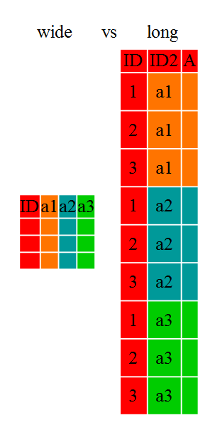
Wide data is presented with each different data variable in a separate column, whereas long data is presented with one column containing all the values and another column listing the context of the value. There are intermediate values between the extremites of long and short. Most modeling and visualization packages prefer long data to wide data.
There are four basic functions to reshape data in tidyr:
- gather(): turn columns into rows
- spread(): turn rows into columns
- separate(): turn a character column into multiple columns
- unite(): turn multiple character columns into a single column
##Gather Gather takes wide data and makes it long. It does this by taking a column name and making that into a variable (called a key), with the value being the cell contents.
normtimedata %>%
  select(Speaker, Vowel, Nasality, NormTime, RepNo, F1, F2, F3) %>%
  gather(variable, value, c(F1:F3))
## # A tibble: 546,450 x 7
## Speaker Vowel Nasality NormTime RepNo variable value
## <chr> <chr> <chr> <dbl> <int> <chr> <dbl>
## 1 BP02 u nasal 0.1 1 F1 569.
## 2 BP02 u nasal 0.2 1 F1 364.
## 3 BP02 u nasal 0.3 1 F1 373.
## 4 BP02 u nasal 0.4 1 F1 303.
## 5 BP02 u nasal 0.5 1 F1 415.
## 6 BP02 u nasal 0.6 1 F1 336.
## 7 BP02 u nasal 0.7 1 F1 336.
## 8 BP02 u nasal 0.8 1 F1 330.
## 9 BP02 u nasal 0.9 1 F1 302.
## 10 BP02 u nasal 1 1 F1 280.
## # … with 546,440 more rows##Spread Spread is going to take long data and make it wide. Be careful using this! Spread is going to take each value of its second argument (the first argument being the dataset, which if you are using the pipe is implicitly included) and make that into a column, with the value in that column being the value specified in the third arugment.
To use spread, if you have a lot of dependent variables you will end up with a bunch of NAs and your data will look awful. In these cases it’s better to maintain a long format. Another way of dealing with this is to create a new variable that includes the information for both variables.
normtimedata %>% select(c(Speaker, Word:NormTime, F1)) %>% spread(Speaker, F1) %>% arrange(RepNo)## # A tibble: 18,660 x 18
## Word Vowel Nasality RepNo NormTime BP02 BP04 BP05 BP06 BP07 BP09 BP10
## <chr> <chr> <chr> <int> <dbl> <dbl> <dbl> <dbl> <dbl> <dbl> <dbl> <dbl>
## 1 abun… u nasal 1 0.1 569. 335. 206. 354. 459. 670. 361.
## 2 abun… u nasal 1 0.2 364. 345. 395. 311. 461. 682. 308.
## 3 abun… u nasal 1 0.3 373. 302. 249. 336. 468. 753. 368.
## 4 abun… u nasal 1 0.4 303. 291. 409. 297. 457. 773. 382.
## 5 abun… u nasal 1 0.5 415. 289. 304. 304. 441. 765. 312.
## 6 abun… u nasal 1 0.6 336. 341. 334. 275. 454. 758. 315.
## 7 abun… u nasal 1 0.7 336. 372. 302. 285. 491. 762. 303.
## 8 abun… u nasal 1 0.8 330. 338. 307. 288. 359. 781. 291.
## 9 abun… u nasal 1 0.9 302. 304. 263. 270. 365. 775. 288.
## 10 abun… u nasal 1 1 280. 285. 287. 269. 291. 756. 276.
## # … with 18,650 more rows, and 6 more variables: BP14 <dbl>, BP17 <dbl>,
## # BP18 <dbl>, BP19 <dbl>, BP20 <dbl>, BP21 <dbl>normtimedata %>% filter(NormTime==0.5) %>% select(c(Speaker, Word:NormTime, F1)) %>% spread(Speaker, F1) %>% arrange(RepNo)## # A tibble: 1,866 x 18
## Word Vowel Nasality RepNo NormTime BP02 BP04 BP05 BP06 BP07 BP09 BP10
## <chr> <chr> <chr> <int> <dbl> <dbl> <dbl> <dbl> <dbl> <dbl> <dbl> <dbl>
## 1 abun… u nasal 1 0.5 415. 289. 304. 304. 441. 765. 312.
## 2 baba… a oral 1 0.5 673. 735. 535. 560. 676. 699. 682.
## 3 bebum u nasal_f… 1 0.5 368. 334. 273. 254. 349. 309. 370.
## 4 cabi… i oral 1 0.5 248. 299. 276. 311. 414. 367. 278.
## 5 cabi… i nasaliz… 1 0.5 312. 326. 279. 261. 327. 371. 277.
## 6 cupim i nasal_f… 1 0.5 311. 361. 280. 275. 391. 1847. 313.
## 7 prop… a nasaliz… 1 0.5 534. 489. 522. 458. 537. 605. 457.
## 8 subi… i nasal 1 0.5 289. 349. 268. 278. 400. 292. 381.
## 9 tapa… a nasal 1 0.5 335. 462. 389. 395. 487. 577. 345.
## 10 trib… u nasaliz… 1 0.5 573. 339. 298. 298. 376. 652. 353.
## # … with 1,856 more rows, and 6 more variables: BP14 <dbl>, BP17 <dbl>,
## # BP18 <dbl>, BP19 <dbl>, BP20 <dbl>, BP21 <dbl>normtimedata %>%
select(Speaker, Vowel, Nasality, NormTime, RepNo, F1, F2, F3) %>%
gather(variable, value, c(F1:F3)) %>%
unite(temp, Speaker, variable) %>%
spread(NormTime, value)## # A tibble: 54,645 x 14
## temp Vowel Nasality RepNo `0.1` `0.2` `0.3` `0.4` `0.5` `0.6` `0.7` `0.8`
## <chr> <chr> <chr> <int> <dbl> <dbl> <dbl> <dbl> <dbl> <dbl> <dbl> <dbl>
## 1 BP02… a nasal 1 460. 464. 433. 337. 335. 326. 331. 345.
## 2 BP02… a nasal 2 471. 473. 433. 443. 363. 345. 341. 332.
## 3 BP02… a nasal 3 496. 491. 466. 357. 209. 273. 253. 306.
## 4 BP02… a nasal 4 521. 480. 483. 374. 1182. 245. 274. 252.
## 5 BP02… a nasal 5 490. 483. 470. 400. 283. 243. 282. 269.
## 6 BP02… a nasal 6 443. 455. 456. 409. 374. 303. 327. 343.
## 7 BP02… a nasal 7 446. 460. 426. 432. 346. 273. 285. 302.
## 8 BP02… a nasal 8 491. 487. 477. 427. 398. 280. 283. 287.
## 9 BP02… a nasal 9 470. 481. 418. 328. 319. 289. 288. 308.
## 10 BP02… a nasal 10 425. 439. 445. 420. 192. 225. 241. 297.
## # … with 54,635 more rows, and 2 more variables: `0.9` <dbl>, `1` <dbl>Separate
Let’s say you want to take information out of a column and make it into multiple columns (similar to the ‘text to columns’ command in Excel). You can use the separate() function to do this.
By default, separate will separate based on any non-alphanumeric character. You can also specify the separater with sep = “____”. You can also specify the number of characters to separate by.
normtimedata %>% separate(Speaker, into = c("Language", "ID"), 2)## # A tibble: 182,150 x 14
## Language ID Word Vowel Nasality RepNo NormTime Type label Time F1
## <chr> <chr> <chr> <chr> <chr> <int> <dbl> <chr> <chr> <dbl> <dbl>
## 1 BP 02 abun… u nasal 1 0.1 clean un 3.39 569.
## 2 BP 02 abun… u nasal 1 0.2 clean un 3.41 364.
## 3 BP 02 abun… u nasal 1 0.3 clean un 3.43 373.
## 4 BP 02 abun… u nasal 1 0.4 clean un 3.46 303.
## 5 BP 02 abun… u nasal 1 0.5 clean un 3.48 415.
## 6 BP 02 abun… u nasal 1 0.6 clean un 3.51 336.
## 7 BP 02 abun… u nasal 1 0.7 clean un 3.53 336.
## 8 BP 02 abun… u nasal 1 0.8 clean un 3.56 330.
## 9 BP 02 abun… u nasal 1 0.9 clean un 3.58 302.
## 10 BP 02 abun… u nasal 1 1 clean un 3.60 280.
## # … with 182,140 more rows, and 3 more variables: F2 <dbl>, F3 <dbl>,
## # F2_3 <dbl>Unite
The opposite of separate is ‘unite’, which will make a new variable out of two variables. Note that for separate and unite, you end getting rid of the old variables.
normtimedata %>% unite(VowNas, Vowel, Nasality, sep = "_")## # A tibble: 182,150 x 12
## Speaker Word VowNas RepNo NormTime Type label Time F1 F2 F3 F2_3
## <chr> <chr> <chr> <int> <dbl> <chr> <chr> <dbl> <dbl> <dbl> <dbl> <dbl>
## 1 BP02 abun… u_nas… 1 0.1 clean un 3.39 569. 2372. 3130. 379.
## 2 BP02 abun… u_nas… 1 0.2 clean un 3.41 364. 2297. 2692. 197.
## 3 BP02 abun… u_nas… 1 0.3 clean un 3.43 373. 2258. 2882. 312.
## 4 BP02 abun… u_nas… 1 0.4 clean un 3.46 303. 2165. 2918. 376.
## 5 BP02 abun… u_nas… 1 0.5 clean un 3.48 415. 2247. 2893. 323.
## 6 BP02 abun… u_nas… 1 0.6 clean un 3.51 336. 2098. 2623. 263.
## 7 BP02 abun… u_nas… 1 0.7 clean un 3.53 336. 2272. 2869. 299.
## 8 BP02 abun… u_nas… 1 0.8 clean un 3.56 330. 1719. 2435. 358.
## 9 BP02 abun… u_nas… 1 0.9 clean un 3.58 302. 2337. 2391. 26.7
## 10 BP02 abun… u_nas… 1 1 clean un 3.60 280. 966. 2435. 734.
## # … with 182,140 more rowsnormtimedata %>% unite(MERP, Speaker, Vowel, Nasality, sep = "!")## # A tibble: 182,150 x 11
## MERP Word RepNo NormTime Type label Time F1 F2 F3 F2_3
## <chr> <chr> <int> <dbl> <chr> <chr> <dbl> <dbl> <dbl> <dbl> <dbl>
## 1 BP02!u!nasal abunda 1 0.1 clean un 3.39 569. 2372. 3130. 379.
## 2 BP02!u!nasal abunda 1 0.2 clean un 3.41 364. 2297. 2692. 197.
## 3 BP02!u!nasal abunda 1 0.3 clean un 3.43 373. 2258. 2882. 312.
## 4 BP02!u!nasal abunda 1 0.4 clean un 3.46 303. 2165. 2918. 376.
## 5 BP02!u!nasal abunda 1 0.5 clean un 3.48 415. 2247. 2893. 323.
## 6 BP02!u!nasal abunda 1 0.6 clean un 3.51 336. 2098. 2623. 263.
## 7 BP02!u!nasal abunda 1 0.7 clean un 3.53 336. 2272. 2869. 299.
## 8 BP02!u!nasal abunda 1 0.8 clean un 3.56 330. 1719. 2435. 358.
## 9 BP02!u!nasal abunda 1 0.9 clean un 3.58 302. 2337. 2391. 26.7
## 10 BP02!u!nasal abunda 1 1 clean un 3.60 280. 966. 2435. 734.
## # … with 182,140 more rows#Relating different data sets with dplyr There are many datasets, especially once you get into larger experiments, that involve the use of multiple tables at once. For these datasets, we need to use a set of tools that relates these tables to one another. There is a great cheat sheet found here to further explain these joins. You can also find more information in R4DS.
In order to show you how different types of joins work, I have included another set of data. It is output from a second set of Praat scripts, which were run to gather further acoustic measures related to nasality (see Styler 2017 for more information). This set of scripts was run at 5 normalized time points, rather than 10, throughout the vowels’ durations.
nasalitydata## # A tibble: 32,145 x 34
## Speaker Word Vowel Nasality RepNo NormTime freq_f1 amp_f1 width_f1 freq_f2
## <chr> <chr> <chr> <chr> <int> <dbl> <dbl> <dbl> <dbl> <dbl>
## 1 BP02 abun… u nasal 1 0.2 352 13.9 680 557
## 2 BP02 abun… u nasal 1 0.4 469 13.1 133 2232
## 3 BP02 abun… u nasal 1 0.6 258 17.6 222 1253
## 4 BP02 abun… u nasal 1 0.8 281 15.7 103 1395
## 5 BP02 abun… u nasal 1 1 141 16.7 53 1220
## 6 BP02 abun… u nasal 2 0.2 422 13.1 120 2196
## 7 BP02 abun… u nasal 2 0.4 211 18.0 139 1324
## 8 BP02 abun… u nasal 2 0.6 234 18.2 140 1156
## 9 BP02 abun… u nasal 2 0.8 258 17.0 143 1609
## 10 BP02 abun… u nasal 2 1 258 17.0 57 860
## # … with 32,135 more rows, and 24 more variables: amp_f2 <dbl>, width_f2 <dbl>,
## # freq_f3 <dbl>, amp_f3 <dbl>, width_f3 <dbl>, freq_h1 <dbl>, amp_h1 <dbl>,
## # freq_h2 <dbl>, amp_h2 <dbl>, amp_h3 <dbl>, amp_p0 <dbl>, freq_p0 <dbl>,
## # p0_id <chr>, p0prominence <dbl>, a1p0_h1 <dbl>, a1p0_h2 <dbl>,
## # a1p0_h3 <dbl>, a1p0 <dbl>, a1p0_compensated <dbl>, freq_p1 <dbl>,
## # amp_p1 <dbl>, a1p1 <dbl>, a1p1_compensated <dbl>, a3p0 <dbl>I will be making subsets of the datasets, which I will show you, in order to demonstrate these joins.
There are two types of joins, and a few differeny options for these types of join:
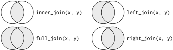
- Mutating joins combine variables from two data frames in a variety of ways.
- left_join(a, b, by = c(‘…’)) - join matching rows from b to a by matching variables in vector
- right_join(a, b, by = c(‘…’)) - join matching rows from a to b by matching variables in vector
- inner_join(a, b, by = c(‘…’)) - join data, retaining only rows in both a and b
- full_join(a, b, by = c(‘…’)) - join data, retaining all values, all rows
- Filtering joins match observations in two data frames, but only affect the observations, rather than the variables.
- semi_join(a, b) keeps all observations in a that have a match in b.
- anti_join(a b) drops all observations in a that have a match in b.
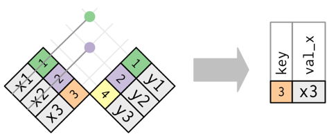
##Mutating Joins
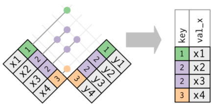
First, we have an inner join. An inner join will only retain rows in both datasets.
nasalitydata %>% filter(Speaker =="BP02") %>% inner_join(normtimedata)## Joining, by = c("Speaker", "Word", "Vowel", "Nasality", "RepNo", "NormTime")## # A tibble: 2,025 x 41
## Speaker Word Vowel Nasality RepNo NormTime freq_f1 amp_f1 width_f1 freq_f2
## <chr> <chr> <chr> <chr> <int> <dbl> <dbl> <dbl> <dbl> <dbl>
## 1 BP02 abun… u nasal 1 0.2 352 13.9 680 557
## 2 BP02 abun… u nasal 1 0.4 469 13.1 133 2232
## 3 BP02 abun… u nasal 1 0.6 258 17.6 222 1253
## 4 BP02 abun… u nasal 1 0.8 281 15.7 103 1395
## 5 BP02 abun… u nasal 1 1 141 16.7 53 1220
## 6 BP02 abun… u nasal 2 0.2 422 13.1 120 2196
## 7 BP02 abun… u nasal 2 0.4 211 18.0 139 1324
## 8 BP02 abun… u nasal 2 0.6 234 18.2 140 1156
## 9 BP02 abun… u nasal 2 0.8 258 17.0 143 1609
## 10 BP02 abun… u nasal 2 1 258 17.0 57 860
## # … with 2,015 more rows, and 31 more variables: amp_f2 <dbl>, width_f2 <dbl>,
## # freq_f3 <dbl>, amp_f3 <dbl>, width_f3 <dbl>, freq_h1 <dbl>, amp_h1 <dbl>,
## # freq_h2 <dbl>, amp_h2 <dbl>, amp_h3 <dbl>, amp_p0 <dbl>, freq_p0 <dbl>,
## # p0_id <chr>, p0prominence <dbl>, a1p0_h1 <dbl>, a1p0_h2 <dbl>,
## # a1p0_h3 <dbl>, a1p0 <dbl>, a1p0_compensated <dbl>, freq_p1 <dbl>,
## # amp_p1 <dbl>, a1p1 <dbl>, a1p1_compensated <dbl>, a3p0 <dbl>, Type <chr>,
## # label <chr>, Time <dbl>, F1 <dbl>, F2 <dbl>, F3 <dbl>, F2_3 <dbl>nasalitydata %>% filter(Speaker =="BP21", RepNo < 20) %>% inner_join(filter(normtimedata, RepNo > 10))## Joining, by = c("Speaker", "Word", "Vowel", "Nasality", "RepNo", "NormTime")## # A tibble: 540 x 41
## Speaker Word Vowel Nasality RepNo NormTime freq_f1 amp_f1 width_f1 freq_f2
## <chr> <chr> <chr> <chr> <int> <dbl> <dbl> <dbl> <dbl> <dbl>
## 1 BP21 abun… u nasal 11 0.2 211 25.2 142 906
## 2 BP21 abun… u nasal 11 0.4 422 24.0 79 846
## 3 BP21 abun… u nasal 11 0.6 234 24.7 129 833
## 4 BP21 abun… u nasal 11 0.8 234 25.6 158 897
## 5 BP21 abun… u nasal 11 1 211 26.1 398 530
## 6 BP21 abun… u nasal 12 0.2 211 22.0 120 850
## 7 BP21 abun… u nasal 12 0.4 211 22.4 103 829
## 8 BP21 abun… u nasal 12 0.6 211 24.3 125 752
## 9 BP21 abun… u nasal 12 0.8 211 24.2 131 872
## 10 BP21 abun… u nasal 12 1 211 24.3 242 427
## # … with 530 more rows, and 31 more variables: amp_f2 <dbl>, width_f2 <dbl>,
## # freq_f3 <dbl>, amp_f3 <dbl>, width_f3 <dbl>, freq_h1 <dbl>, amp_h1 <dbl>,
## # freq_h2 <dbl>, amp_h2 <dbl>, amp_h3 <dbl>, amp_p0 <dbl>, freq_p0 <dbl>,
## # p0_id <chr>, p0prominence <dbl>, a1p0_h1 <dbl>, a1p0_h2 <dbl>,
## # a1p0_h3 <dbl>, a1p0 <dbl>, a1p0_compensated <dbl>, freq_p1 <dbl>,
## # amp_p1 <dbl>, a1p1 <dbl>, a1p1_compensated <dbl>, a3p0 <dbl>, Type <chr>,
## # label <chr>, Time <dbl>, F1 <dbl>, F2 <dbl>, F3 <dbl>, F2_3 <dbl>Whereas an inner join keeps observations in both datasets, outer joins keeps observations that exist in at least one dataset. There are three types of outer joins: left joins, right joins, and full joins.
A left join will retain all observations that are in the first dataset. Conversely, a right join will retain all observations that are in the second dataset. These joins work by adding an additional “virtual” observation to each table. This observation has a key that always matches (if no other key matches), and a value filled with NA. A left join will be more common to use in the “wild.”
dim(nasalitydata)## [1] 32145 34dim(normtimedata)## [1] 182150 13nasalitydata %>% left_join(normtimedata)## Joining, by = c("Speaker", "Word", "Vowel", "Nasality", "RepNo", "NormTime")## # A tibble: 32,145 x 41
## Speaker Word Vowel Nasality RepNo NormTime freq_f1 amp_f1 width_f1 freq_f2
## <chr> <chr> <chr> <chr> <int> <dbl> <dbl> <dbl> <dbl> <dbl>
## 1 BP02 abun… u nasal 1 0.2 352 13.9 680 557
## 2 BP02 abun… u nasal 1 0.4 469 13.1 133 2232
## 3 BP02 abun… u nasal 1 0.6 258 17.6 222 1253
## 4 BP02 abun… u nasal 1 0.8 281 15.7 103 1395
## 5 BP02 abun… u nasal 1 1 141 16.7 53 1220
## 6 BP02 abun… u nasal 2 0.2 422 13.1 120 2196
## 7 BP02 abun… u nasal 2 0.4 211 18.0 139 1324
## 8 BP02 abun… u nasal 2 0.6 234 18.2 140 1156
## 9 BP02 abun… u nasal 2 0.8 258 17.0 143 1609
## 10 BP02 abun… u nasal 2 1 258 17.0 57 860
## # … with 32,135 more rows, and 31 more variables: amp_f2 <dbl>, width_f2 <dbl>,
## # freq_f3 <dbl>, amp_f3 <dbl>, width_f3 <dbl>, freq_h1 <dbl>, amp_h1 <dbl>,
## # freq_h2 <dbl>, amp_h2 <dbl>, amp_h3 <dbl>, amp_p0 <dbl>, freq_p0 <dbl>,
## # p0_id <chr>, p0prominence <dbl>, a1p0_h1 <dbl>, a1p0_h2 <dbl>,
## # a1p0_h3 <dbl>, a1p0 <dbl>, a1p0_compensated <dbl>, freq_p1 <dbl>,
## # amp_p1 <dbl>, a1p1 <dbl>, a1p1_compensated <dbl>, a3p0 <dbl>, Type <chr>,
## # label <chr>, Time <dbl>, F1 <dbl>, F2 <dbl>, F3 <dbl>, F2_3 <dbl>normtimedata %>% filter(NormTime ==0.3) %>% left_join(nasalitydata)## Joining, by = c("Speaker", "Word", "Vowel", "Nasality", "RepNo", "NormTime")## # A tibble: 18,215 x 41
## Speaker Word Vowel Nasality RepNo NormTime Type label Time F1 F2
## <chr> <chr> <chr> <chr> <int> <dbl> <chr> <chr> <dbl> <dbl> <dbl>
## 1 BP02 abun… u nasal 1 0.3 clean un 3.43 373. 2258.
## 2 BP02 abun… u nasal 2 0.3 clean un 5.86 287. 1767.
## 3 BP02 abun… u nasal 3 0.3 clean un 8.46 321. 2249.
## 4 BP02 abun… u nasal 4 0.3 clean un 11.2 347. 977.
## 5 BP02 abun… u nasal 5 0.3 clean un 14.0 369. 1342.
## 6 BP02 abun… u nasal 6 0.3 clean un 16.3 352. 2245.
## 7 BP02 abun… u nasal 7 0.3 clean un 18.9 278. 1958.
## 8 BP02 abun… u nasal 8 0.3 clean un 21.7 272. 1696.
## 9 BP02 abun… u nasal 9 0.3 clean un 24.5 399. 2166.
## 10 BP02 abun… u nasal 10 0.3 clean un 27.2 343. 1389.
## # … with 18,205 more rows, and 30 more variables: F3 <dbl>, F2_3 <dbl>,
## # freq_f1 <dbl>, amp_f1 <dbl>, width_f1 <dbl>, freq_f2 <dbl>, amp_f2 <dbl>,
## # width_f2 <dbl>, freq_f3 <dbl>, amp_f3 <dbl>, width_f3 <dbl>, freq_h1 <dbl>,
## # amp_h1 <dbl>, freq_h2 <dbl>, amp_h2 <dbl>, amp_h3 <dbl>, amp_p0 <dbl>,
## # freq_p0 <dbl>, p0_id <chr>, p0prominence <dbl>, a1p0_h1 <dbl>,
## # a1p0_h2 <dbl>, a1p0_h3 <dbl>, a1p0 <dbl>, a1p0_compensated <dbl>,
## # freq_p1 <dbl>, amp_p1 <dbl>, a1p1 <dbl>, a1p1_compensated <dbl>, a3p0 <dbl>nasalitydata %>% filter(NormTime ==0.2, Vowel =="a") %>% left_join(normtimedata)## Joining, by = c("Speaker", "Word", "Vowel", "Nasality", "RepNo", "NormTime")## # A tibble: 2,155 x 41
## Speaker Word Vowel Nasality RepNo NormTime freq_f1 amp_f1 width_f1 freq_f2
## <chr> <chr> <chr> <chr> <int> <dbl> <dbl> <dbl> <dbl> <dbl>
## 1 BP02 baba… a oral 1 0.2 539 16.2 100 1078
## 2 BP02 baba… a oral 2 0.2 586 20.5 63 1148
## 3 BP02 baba… a oral 3 0.2 633 18.0 64 1128
## 4 BP02 baba… a oral 4 0.2 633 20.3 81 1154
## 5 BP02 baba… a oral 5 0.2 633 19.9 45 1101
## 6 BP02 baba… a oral 6 0.2 633 20.2 46 1107
## 7 BP02 baba… a oral 7 0.2 633 19.9 53 1133
## 8 BP02 baba… a oral 8 0.2 586 18.7 58 1089
## 9 BP02 baba… a oral 9 0.2 609 15.7 63 1055
## 10 BP02 baba… a oral 10 0.2 586 18.9 49 1117
## # … with 2,145 more rows, and 31 more variables: amp_f2 <dbl>, width_f2 <dbl>,
## # freq_f3 <dbl>, amp_f3 <dbl>, width_f3 <dbl>, freq_h1 <dbl>, amp_h1 <dbl>,
## # freq_h2 <dbl>, amp_h2 <dbl>, amp_h3 <dbl>, amp_p0 <dbl>, freq_p0 <dbl>,
## # p0_id <chr>, p0prominence <dbl>, a1p0_h1 <dbl>, a1p0_h2 <dbl>,
## # a1p0_h3 <dbl>, a1p0 <dbl>, a1p0_compensated <dbl>, freq_p1 <dbl>,
## # amp_p1 <dbl>, a1p1 <dbl>, a1p1_compensated <dbl>, a3p0 <dbl>, Type <chr>,
## # label <chr>, Time <dbl>, F1 <dbl>, F2 <dbl>, F3 <dbl>, F2_3 <dbl>nasalitydata %>% filter(NormTime == 0.2, Vowel =="u") %>% right_join(normtimedata)## Joining, by = c("Speaker", "Word", "Vowel", "Nasality", "RepNo", "NormTime")## # A tibble: 182,150 x 41
## Speaker Word Vowel Nasality RepNo NormTime freq_f1 amp_f1 width_f1 freq_f2
## <chr> <chr> <chr> <chr> <int> <dbl> <dbl> <dbl> <dbl> <dbl>
## 1 BP02 abun… u nasal 1 0.2 352 13.9 680 557
## 2 BP02 abun… u nasal 2 0.2 422 13.1 120 2196
## 3 BP02 abun… u nasal 3 0.2 398 12.6 121 2268
## 4 BP02 abun… u nasal 4 0.2 422 13.9 1311 504
## 5 BP02 abun… u nasal 5 0.2 445 13.1 131 1754
## 6 BP02 abun… u nasal 6 0.2 398 14.9 186 551
## 7 BP02 abun… u nasal 7 0.2 305 9.55 303 618
## 8 BP02 abun… u nasal 8 0.2 422 10.7 656 530
## 9 BP02 abun… u nasal 9 0.2 211 16.1 212 674
## 10 BP02 abun… u nasal 10 0.2 398 14.0 166 679
## # … with 182,140 more rows, and 31 more variables: amp_f2 <dbl>,
## # width_f2 <dbl>, freq_f3 <dbl>, amp_f3 <dbl>, width_f3 <dbl>, freq_h1 <dbl>,
## # amp_h1 <dbl>, freq_h2 <dbl>, amp_h2 <dbl>, amp_h3 <dbl>, amp_p0 <dbl>,
## # freq_p0 <dbl>, p0_id <chr>, p0prominence <dbl>, a1p0_h1 <dbl>,
## # a1p0_h2 <dbl>, a1p0_h3 <dbl>, a1p0 <dbl>, a1p0_compensated <dbl>,
## # freq_p1 <dbl>, amp_p1 <dbl>, a1p1 <dbl>, a1p1_compensated <dbl>,
## # a3p0 <dbl>, Type <chr>, label <chr>, Time <dbl>, F1 <dbl>, F2 <dbl>,
## # F3 <dbl>, F2_3 <dbl>The last type of outer join is a full join. It keeps all observations from both datasets. Remember when using the pipe that the argument that goes into full join is on the left hand side of the full_join() function, so if you do any filtering, keep that in mind!
normtimedata %>% full_join(nasalitydata)## Joining, by = c("Speaker", "Word", "Vowel", "Nasality", "RepNo", "NormTime")## # A tibble: 182,155 x 41
## Speaker Word Vowel Nasality RepNo NormTime Type label Time F1 F2
## <chr> <chr> <chr> <chr> <int> <dbl> <chr> <chr> <dbl> <dbl> <dbl>
## 1 BP02 abun… u nasal 1 0.1 clean un 3.39 569. 2372.
## 2 BP02 abun… u nasal 1 0.2 clean un 3.41 364. 2297.
## 3 BP02 abun… u nasal 1 0.3 clean un 3.43 373. 2258.
## 4 BP02 abun… u nasal 1 0.4 clean un 3.46 303. 2165.
## 5 BP02 abun… u nasal 1 0.5 clean un 3.48 415. 2247.
## 6 BP02 abun… u nasal 1 0.6 clean un 3.51 336. 2098.
## 7 BP02 abun… u nasal 1 0.7 clean un 3.53 336. 2272.
## 8 BP02 abun… u nasal 1 0.8 clean un 3.56 330. 1719.
## 9 BP02 abun… u nasal 1 0.9 clean un 3.58 302. 2337.
## 10 BP02 abun… u nasal 1 1 clean un 3.60 280. 966.
## # … with 182,145 more rows, and 30 more variables: F3 <dbl>, F2_3 <dbl>,
## # freq_f1 <dbl>, amp_f1 <dbl>, width_f1 <dbl>, freq_f2 <dbl>, amp_f2 <dbl>,
## # width_f2 <dbl>, freq_f3 <dbl>, amp_f3 <dbl>, width_f3 <dbl>, freq_h1 <dbl>,
## # amp_h1 <dbl>, freq_h2 <dbl>, amp_h2 <dbl>, amp_h3 <dbl>, amp_p0 <dbl>,
## # freq_p0 <dbl>, p0_id <chr>, p0prominence <dbl>, a1p0_h1 <dbl>,
## # a1p0_h2 <dbl>, a1p0_h3 <dbl>, a1p0 <dbl>, a1p0_compensated <dbl>,
## # freq_p1 <dbl>, amp_p1 <dbl>, a1p1 <dbl>, a1p1_compensated <dbl>, a3p0 <dbl>normtimedata %>% filter(NormTime == 0.4) %>% full_join(nasalitydata) %>% arrange(Speaker, Vowel, Nasality, RepNo, NormTime) ## Joining, by = c("Speaker", "Word", "Vowel", "Nasality", "RepNo", "NormTime")## # A tibble: 43,932 x 41
## Speaker Word Vowel Nasality RepNo NormTime Type label Time F1 F2
## <chr> <chr> <chr> <chr> <int> <dbl> <chr> <chr> <dbl> <dbl> <dbl>
## 1 BP02 tapa… a nasal 1 0.2 <NA> <NA> NA NA NA
## 2 BP02 tapa… a nasal 1 0.4 clean an 3.67 337. 1734.
## 3 BP02 tapa… a nasal 1 0.6 <NA> <NA> NA NA NA
## 4 BP02 tapa… a nasal 1 0.8 <NA> <NA> NA NA NA
## 5 BP02 tapa… a nasal 1 1 <NA> <NA> NA NA NA
## 6 BP02 tapa… a nasal 2 0.2 <NA> <NA> NA NA NA
## 7 BP02 tapa… a nasal 2 0.4 clean an 6.22 443. 1966.
## 8 BP02 tapa… a nasal 2 0.6 <NA> <NA> NA NA NA
## 9 BP02 tapa… a nasal 2 0.8 <NA> <NA> NA NA NA
## 10 BP02 tapa… a nasal 2 1 <NA> <NA> NA NA NA
## # … with 43,922 more rows, and 30 more variables: F3 <dbl>, F2_3 <dbl>,
## # freq_f1 <dbl>, amp_f1 <dbl>, width_f1 <dbl>, freq_f2 <dbl>, amp_f2 <dbl>,
## # width_f2 <dbl>, freq_f3 <dbl>, amp_f3 <dbl>, width_f3 <dbl>, freq_h1 <dbl>,
## # amp_h1 <dbl>, freq_h2 <dbl>, amp_h2 <dbl>, amp_h3 <dbl>, amp_p0 <dbl>,
## # freq_p0 <dbl>, p0_id <chr>, p0prominence <dbl>, a1p0_h1 <dbl>,
## # a1p0_h2 <dbl>, a1p0_h3 <dbl>, a1p0 <dbl>, a1p0_compensated <dbl>,
## # freq_p1 <dbl>, amp_p1 <dbl>, a1p1 <dbl>, a1p1_compensated <dbl>, a3p0 <dbl>Why does the second example here only have NormTime values of 0.2, 0.4, 0.6, 0.8, and 1?
##Filtering joins Unlike mutating joins, filtering joins do not combine multiple datasets. They only affect the observations from the first dataset. (You can think of it as using data that is or isn’t in the second set to filter the first set, based ona particular key.)
A semi join will keep all observations in the first dataset which have a match in the second dataset. An anti join will discard these observations, and will only keep the observations in the first dataset that don’t have a match in the second set.
normtimedata %>% semi_join(nasalitydata)## Joining, by = c("Speaker", "Word", "Vowel", "Nasality", "RepNo", "NormTime")## # A tibble: 32,140 x 13
## Speaker Word Vowel Nasality RepNo NormTime Type label Time F1 F2
## <chr> <chr> <chr> <chr> <int> <dbl> <chr> <chr> <dbl> <dbl> <dbl>
## 1 BP02 abun… u nasal 1 0.2 clean un 3.41 364. 2297.
## 2 BP02 abun… u nasal 1 0.4 clean un 3.46 303. 2165.
## 3 BP02 abun… u nasal 1 0.6 clean un 3.51 336. 2098.
## 4 BP02 abun… u nasal 1 0.8 clean un 3.56 330. 1719.
## 5 BP02 abun… u nasal 1 1 clean un 3.60 280. 966.
## 6 BP02 abun… u nasal 2 0.2 clean un 5.83 326. 2185.
## 7 BP02 abun… u nasal 2 0.4 clean un 5.88 334. 1471.
## 8 BP02 abun… u nasal 2 0.6 clean un 5.93 310. 1371.
## 9 BP02 abun… u nasal 2 0.8 clean un 5.97 306. 1308.
## 10 BP02 abun… u nasal 2 1 clean un 6.02 305. 2169.
## # … with 32,130 more rows, and 2 more variables: F3 <dbl>, F2_3 <dbl>nasalitydata %>% semi_join(normtimedata)## Joining, by = c("Speaker", "Word", "Vowel", "Nasality", "RepNo", "NormTime")## # A tibble: 32,140 x 34
## Speaker Word Vowel Nasality RepNo NormTime freq_f1 amp_f1 width_f1 freq_f2
## <chr> <chr> <chr> <chr> <int> <dbl> <dbl> <dbl> <dbl> <dbl>
## 1 BP02 abun… u nasal 1 0.2 352 13.9 680 557
## 2 BP02 abun… u nasal 1 0.4 469 13.1 133 2232
## 3 BP02 abun… u nasal 1 0.6 258 17.6 222 1253
## 4 BP02 abun… u nasal 1 0.8 281 15.7 103 1395
## 5 BP02 abun… u nasal 1 1 141 16.7 53 1220
## 6 BP02 abun… u nasal 2 0.2 422 13.1 120 2196
## 7 BP02 abun… u nasal 2 0.4 211 18.0 139 1324
## 8 BP02 abun… u nasal 2 0.6 234 18.2 140 1156
## 9 BP02 abun… u nasal 2 0.8 258 17.0 143 1609
## 10 BP02 abun… u nasal 2 1 258 17.0 57 860
## # … with 32,130 more rows, and 24 more variables: amp_f2 <dbl>, width_f2 <dbl>,
## # freq_f3 <dbl>, amp_f3 <dbl>, width_f3 <dbl>, freq_h1 <dbl>, amp_h1 <dbl>,
## # freq_h2 <dbl>, amp_h2 <dbl>, amp_h3 <dbl>, amp_p0 <dbl>, freq_p0 <dbl>,
## # p0_id <chr>, p0prominence <dbl>, a1p0_h1 <dbl>, a1p0_h2 <dbl>,
## # a1p0_h3 <dbl>, a1p0 <dbl>, a1p0_compensated <dbl>, freq_p1 <dbl>,
## # amp_p1 <dbl>, a1p1 <dbl>, a1p1_compensated <dbl>, a3p0 <dbl>normtimedata %>% anti_join(nasalitydata)## Joining, by = c("Speaker", "Word", "Vowel", "Nasality", "RepNo", "NormTime")## # A tibble: 150,010 x 13
## Speaker Word Vowel Nasality RepNo NormTime Type label Time F1 F2
## <chr> <chr> <chr> <chr> <int> <dbl> <chr> <chr> <dbl> <dbl> <dbl>
## 1 BP02 abun… u nasal 1 0.1 clean un 3.39 569. 2372.
## 2 BP02 abun… u nasal 1 0.3 clean un 3.43 373. 2258.
## 3 BP02 abun… u nasal 1 0.5 clean un 3.48 415. 2247.
## 4 BP02 abun… u nasal 1 0.7 clean un 3.53 336. 2272.
## 5 BP02 abun… u nasal 1 0.9 clean un 3.58 302. 2337.
## 6 BP02 abun… u nasal 2 0.1 clean un 5.81 492. 2277.
## 7 BP02 abun… u nasal 2 0.3 clean un 5.86 287. 1767.
## 8 BP02 abun… u nasal 2 0.5 clean un 5.90 367. 2301.
## 9 BP02 abun… u nasal 2 0.7 clean un 5.95 385. 2114.
## 10 BP02 abun… u nasal 2 0.9 clean un 6.00 285. 1020.
## # … with 150,000 more rows, and 2 more variables: F3 <dbl>, F2_3 <dbl>nasalitydata %>% anti_join(normtimedata)## Joining, by = c("Speaker", "Word", "Vowel", "Nasality", "RepNo", "NormTime")## # A tibble: 5 x 34
## Speaker Word Vowel Nasality RepNo NormTime freq_f1 amp_f1 width_f1 freq_f2
## <chr> <chr> <chr> <chr> <int> <dbl> <dbl> <dbl> <dbl> <dbl>
## 1 BP04 trib… <NA> <NA> 44 0.2 164 23.9 77 1110
## 2 BP04 trib… <NA> <NA> 44 0.4 188 18.9 33 1319
## 3 BP04 trib… <NA> <NA> 44 0.6 117 2.71 461 1660
## 4 BP04 trib… <NA> <NA> 44 0.8 234 24.0 36 1210
## 5 BP04 trib… <NA> <NA> 44 1 164 23.2 137 828
## # … with 24 more variables: amp_f2 <dbl>, width_f2 <dbl>, freq_f3 <dbl>,
## # amp_f3 <dbl>, width_f3 <dbl>, freq_h1 <dbl>, amp_h1 <dbl>, freq_h2 <dbl>,
## # amp_h2 <dbl>, amp_h3 <dbl>, amp_p0 <dbl>, freq_p0 <dbl>, p0_id <chr>,
## # p0prominence <dbl>, a1p0_h1 <dbl>, a1p0_h2 <dbl>, a1p0_h3 <dbl>,
## # a1p0 <dbl>, a1p0_compensated <dbl>, freq_p1 <dbl>, amp_p1 <dbl>,
## # a1p1 <dbl>, a1p1_compensated <dbl>, a3p0 <dbl>#As it turns out, there was one dataset in the nasality data that, for some reason, was not calculated in the normtime dataset.#My data processing code This is the processing code I used to get the data from my dissertation out of .txt form and into R. Note that it is not the final version of the data. Rather, it is processed to the point where it can be worked with in this module. Further processing was done, specifically using the select() and filter() verbs, to create my final dataset, which is not shown here.
Some of this is based on methods found on this website.
normtimewd = "/Users/marissabarlaz/Desktop/Work/LING/LING 490/Data/All NormTime Formant"
allfiles = dir(normtimewd, "*.normtime_formant")

normtimedata <- data_frame(filename = allfiles) %>%
  mutate(file_contents = map(filename, ~ read_tsv(file.path(normtimewd, .), skip = 1, col_names = c("label", "Time", "F1", "F2", "F3", "F2_3")))) %>%
  #skip = 1 because there's a problem with the column names
        unnest() %>%
  separate(filename, into = c("Type", "Speaker", "Position", "Word"), extra = "drop") %>%
  mutate(NormTime = (1:length(Time) %%10)*0.1,
         label1 = label)%>%
 separate(label1, into = c("Vowel", "Nasality"), 1) %>%
  select(-c(Position))


normtimedata$NormTime[normtimedata$NormTime ==0.0] = 1
normtimedata$NormTime = as.numeric(trimws(normtimedata$NormTime))

normtimedata$Nasality = plyr::mapvalues(normtimedata$Nasality, from=c("~", "m", "n", "o", "s"), to=c("nasalized","nasal_final", "nasal", "oral", "nasalized"))

normtimedata  = normtimedata %>%
  group_by(Speaker, Word, NormTime) %>%
  mutate(RepNo = seq(n())) %>%
  ungroup() %>%
  select(Speaker, Word, Vowel, Nasality, RepNo, NormTime, everything())


#write_csv(normtimedata, paste(normtimewd, "normtimedata.csv", sep=""))


### NASALITY DATA PROCESSING

nasalitywd = "/Users/marissabarlaz/Desktop/Work/LING/LING 490/Data/Acoustic Nasality Data"
allnasalfiles = dir(nasalitywd, "*.txt")

nasalitydata <- data_frame(filename = allnasalfiles) %>%
  mutate(file_contents = map(filename, ~ read_tsv(file.path(nasalitywd, .), skip = 0))) %>%

        unnest() %>%
  rename(label = vowel) %>%

  separate(filename1, into = c("Speaker", "Position", "Word")) %>%

  mutate(label1 = label,
         NormTime = timepoint/5) %>%
   separate(label1, into = c("Vowel", "Nasality"), 1) %>%
  select(-c("filename", "word", "label", "timepoint", "point_time")) %>%
  select(-c(Position, vwl_amp_rms:errorflag))

nasalitydata$Nasality = plyr::mapvalues(nasalitydata$Nasality, from=c("~", "m", "n", "o", "s"), to=c("nasalized","nasal_final", "nasal", "oral", "nasalized"))


nasalitydata  = nasalitydata %>%
  group_by(Speaker, Word, NormTime) %>%
  mutate(RepNo = seq(n())) %>%
  ungroup() %>%
  select(Speaker, Word, Vowel, Nasality, RepNo, NormTime, everything())

#write_csv(nasalitydata, paste(normtimewd, "nasalitydata_styler_all.csv", sep=""))