Bayesian Analysis in R

What is Bayesian analysis?
- A simple Bayesian analysis
- Why use Bayesian analysis?
How to run a Bayesian analysis in R

The packages I will be using for this workshop include:

library(tidyverse)
library(brms)
library(ggridges)
library(shinystan)
library(bayesplot)
library(tidybayes)
library(ggmcmc)

The data I will be using is a subset of my dissertation data, which looks like this:

head(normtimeBP)

## # A tibble: 6 x 9
## # Groups:   Speaker [1]
##   Speaker Vowel Nasality RepNo NormTime    F1    F2    F3  F2_3
##   <fct>   <fct> <fct>    <fct>    <dbl> <dbl> <dbl> <dbl> <dbl>
## 1 BP02    u     nasal    1          0.5  415. 2247. 2893.  323.
## 2 BP02    u     nasal    2          0.5  367. 2301. 2898.  298.
## 3 BP02    u     nasal    3          0.5  315. 1508. 2549.  521.
## 4 BP02    u     nasal    4          0.5  301. 1369. 2374.  502.
## 5 BP02    u     nasal    5          0.5  336. 1252. 2441.  595.
## 6 BP02    u     nasal    6          0.5  310. 2077. 2696.  309.

str(normtimeBP, give.attr = FALSE)

## tibble [4,655 × 9] (S3: grouped_df/tbl_df/tbl/data.frame)
##  $ Speaker : Factor w/ 12 levels "BP02","BP04",..: 1 1 1 1 1 1 1 1 1 1 ...
##  $ Vowel   : Factor w/ 3 levels "a","i","u": 3 3 3 3 3 3 3 3 3 3 ...
##  $ Nasality: Factor w/ 3 levels "nasal","nasalized",..: 1 1 1 1 1 1 1 1 1 1 ...
##  $ RepNo   : Factor w/ 70 levels "1","2","3","4",..: 1 2 3 4 5 6 7 8 9 10 ...
##  $ NormTime: num [1:4655] 0.5 0.5 0.5 0.5 0.5 0.5 0.5 0.5 0.5 0.5 ...
##  $ F1      : num [1:4655] 415 367 315 301 336 ...
##  $ F2      : num [1:4655] 2247 2301 1508 1369 1252 ...
##  $ F3      : num [1:4655] 2893 2898 2549 2374 2441 ...
##  $ F2_3    : num [1:4655] 323 298 521 502 595 ...

summary(normtimeBP)

##     Speaker     Vowel         Nasality        RepNo         NormTime  
##  BP04   : 608   a:1492   nasal    :1586   6      : 108   Min.   :0.5  
##  BP06   : 508   i:1598   nasalized:1569   23     : 107   1st Qu.:0.5  
##  BP14   : 432   u:1565   oral     :1500   5      : 106   Median :0.5  
##  BP10   : 385                             24     : 106   Mean   :0.5  
##  BP05   : 383                             1      : 105   3rd Qu.:0.5  
##  BP21   : 376                             2      : 105   Max.   :0.5  
##  (Other):1963                             (Other):4018                
##        F1              F2               F3            F2_3        
##  Min.   :200.1   Min.   : 309.7   Min.   :1186   Min.   :  13.99  
##  1st Qu.:307.9   1st Qu.: 963.3   1st Qu.:2564   1st Qu.: 463.80  
##  Median :367.6   Median :1277.4   Median :2856   Median : 693.28  
##  Mean   :399.6   Mean   :1507.5   Mean   :2884   Mean   : 688.40  
##  3rd Qu.:449.3   3rd Qu.:2152.9   3rd Qu.:3197   3rd Qu.: 903.69  
##  Max.   :799.5   Max.   :3212.1   Max.   :4444   Max.   :1495.86  
##

What is Bayesian analysis?

The majority of experimental linguistic research has been analyzed using frequentist statistics - that is, we draw conclusions from our sample data based on the frequency or proportion of groups within the data, and then we attempt to extrapolate to the larger community based on this sample. In these cases, we are often comparing our data to a null hypothesis - is our data compatible with this “no difference” hypothesis? We obtain a p-value, which measures the (in)compatibility of our data with this hypothesis. These methods rely heavily on point values, such as means and medians.

Bayesian inference is an entirely different ballgame. Instead of relying on single points such as means or medians, it is a probability-based system. In this system there is a relationship between previously known information and your current dataset. The output of the analysis includes credible intervals - that is, based on previous information plus your current model, what is the most probable range of values for your variable of interest?

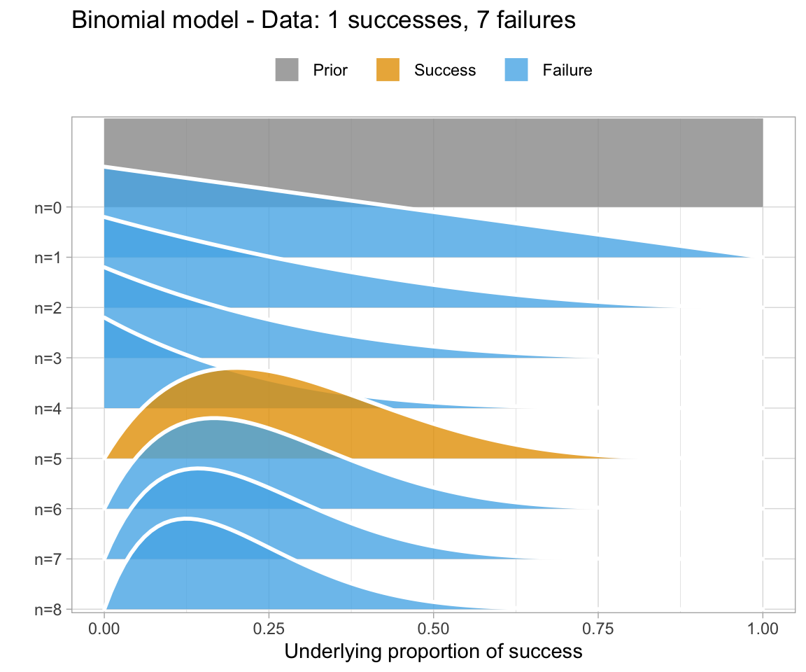
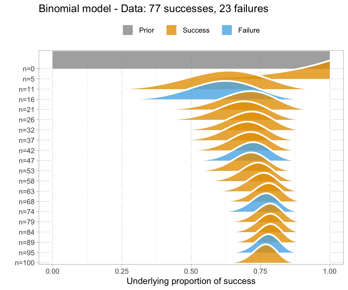
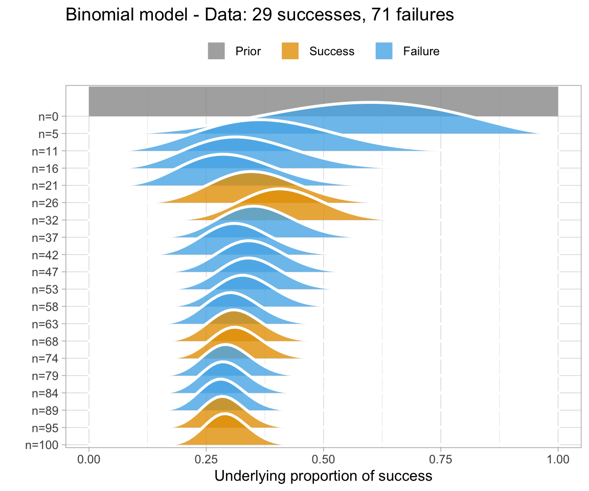
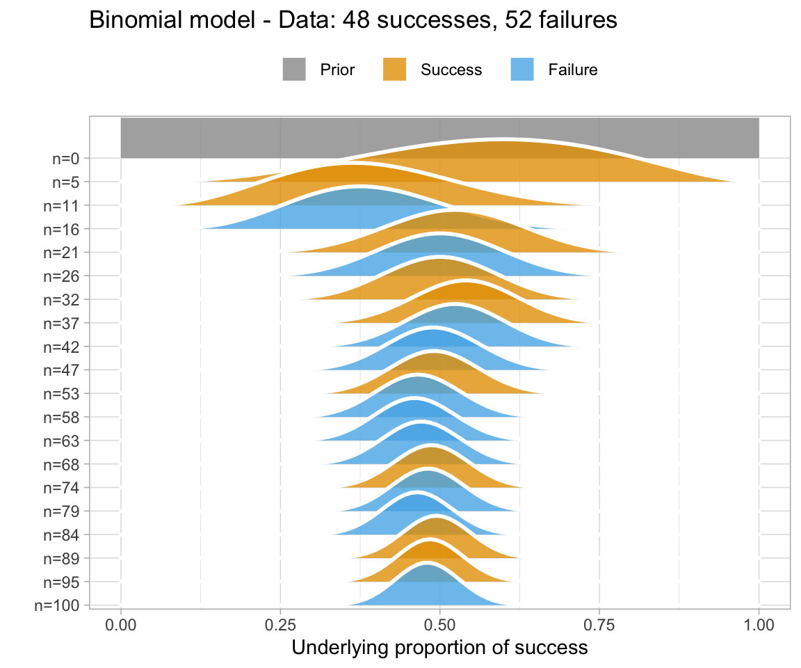
Informally, Bayes’ theorem is: Posterior ∝ Prior × Likelihood.

A simple Bayesian analysis

## Warning: `data_frame()` is deprecated as of tibble 1.1.0.
## Please use `tibble()` instead.
## This warning is displayed once every 8 hours.
## Call `lifecycle::last_warnings()` to see where this warning was generated.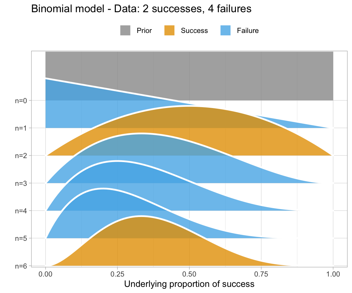

Why use Bayesian analysis?

There are many reasons to use Bayesian analysis instead of frequentist analytics. Bayesian analysis is really flexible in that:

You can include information sources in addition to the data.

this includes background information given in textbooks or previous studies, common knowledge, etc.

You can make any comparisons between groups or data sets.

This is especially important for linguistic research.

Bayesian methods allow us to directly the question we are interested in: How plausible is our hypothesis given the data?

This allows us to quantify uncertainty about the data and avoid terms such as “prove”.

Models are more easily defined and are more flexible, and not susceptible to things such as separation.

How to run a Bayesian analysis in R

There are a bunch of different packages availble for doing Bayesian analysis in R. These include RJAGS and rstanarm, among others. The development of the programming language Stan has made doing Bayesian analysis easier for social sciences. We will use the package brms, which is written to communicate with Stan, and allows us to use syntax analogous to the lme4 package. Note that previous tutorials written for linguistic research use the rstan and rstanarm packages (such as Sorensen, Hohenstein and Vasishth, 2016 and Nicenbolm and Vasishth, 2016). A more recent tutorial (Vasishth et al., 2018) utilizes the brms package.

Vasishth et al. (2018) identify five steps in carrying out an analysis in a Bayesian framework. They are:

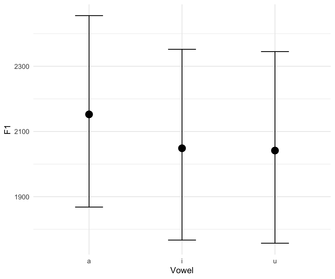
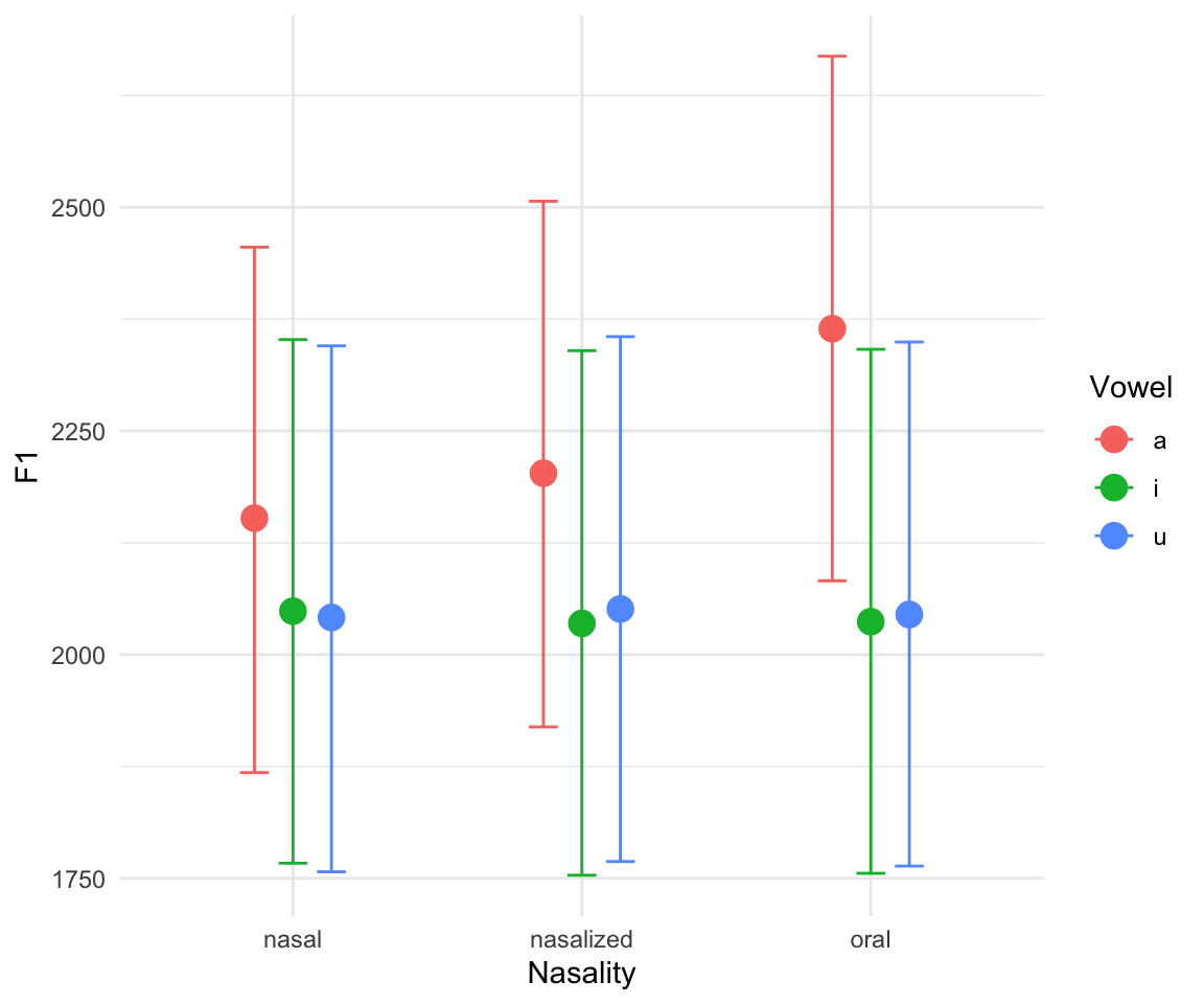
Explore the data using graphical tools; visualize the relationships between variables of interest.
Define model(s) and priors.
Fit model(s) to data.
Check for convergence.
Carry out inference by:

summarizing and displaying posterior distributions
computing Bayes factors with several different priors for theparameter being tested
evaluating predictive performance of competing models using k-fold cross-validation or approximations of leave-one-out cross-validation.

Step 1: Data exploration

summary(normtimeBP)

##     Speaker     Vowel         Nasality        RepNo         NormTime  
##  BP04   : 608   a:1492   nasal    :1586   6      : 108   Min.   :0.5  
##  BP06   : 508   i:1598   nasalized:1569   23     : 107   1st Qu.:0.5  
##  BP14   : 432   u:1565   oral     :1500   5      : 106   Median :0.5  
##  BP10   : 385                             24     : 106   Mean   :0.5  
##  BP05   : 383                             1      : 105   3rd Qu.:0.5  
##  BP21   : 376                             2      : 105   Max.   :0.5  
##  (Other):1963                             (Other):4018                
##        F1              F2               F3            F2_3        
##  Min.   :200.1   Min.   : 309.7   Min.   :1186   Min.   :  13.99  
##  1st Qu.:307.9   1st Qu.: 963.3   1st Qu.:2564   1st Qu.: 463.80  
##  Median :367.6   Median :1277.4   Median :2856   Median : 693.28  
##  Mean   :399.6   Mean   :1507.5   Mean   :2884   Mean   : 688.40  
##  3rd Qu.:449.3   3rd Qu.:2152.9   3rd Qu.:3197   3rd Qu.: 903.69  
##  Max.   :799.5   Max.   :3212.1   Max.   :4444   Max.   :1495.86  
##

ggplot(normtimeBP, aes(x = F1, y = F2, color = Vowel, shape = Nasality)) + geom_point(alpha = 0.2) + scale_color_manual(values = cbPalette) + stat_ellipse(aes(linetype = Nasality))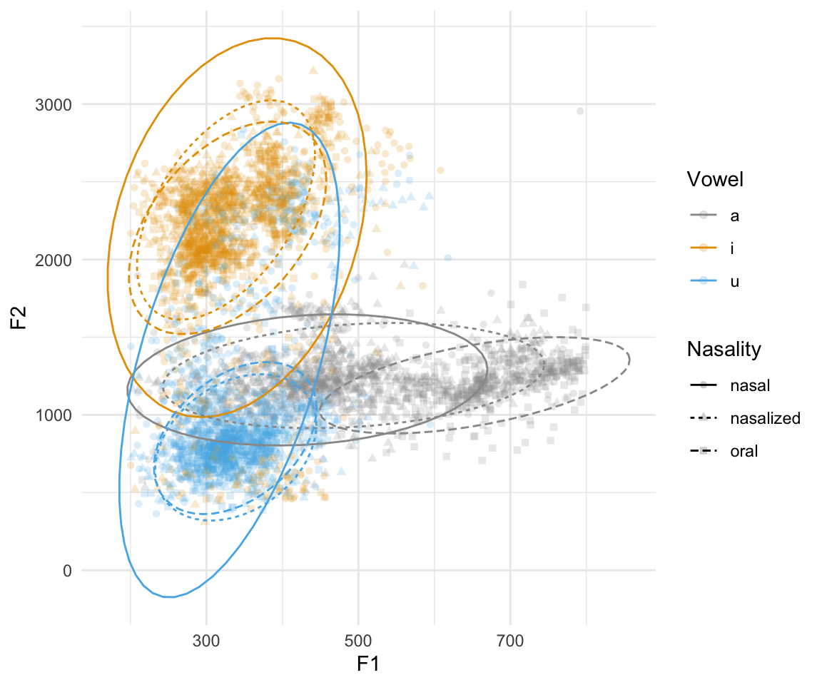

ggplot(normtimeBP, aes(x = F1, color = Nasality, fill = Nasality)) + geom_density(alpha = 0.2) + scale_color_manual(values = cbPalette)+scale_fill_manual(values = cbPalette) +facet_wrap(~Vowel)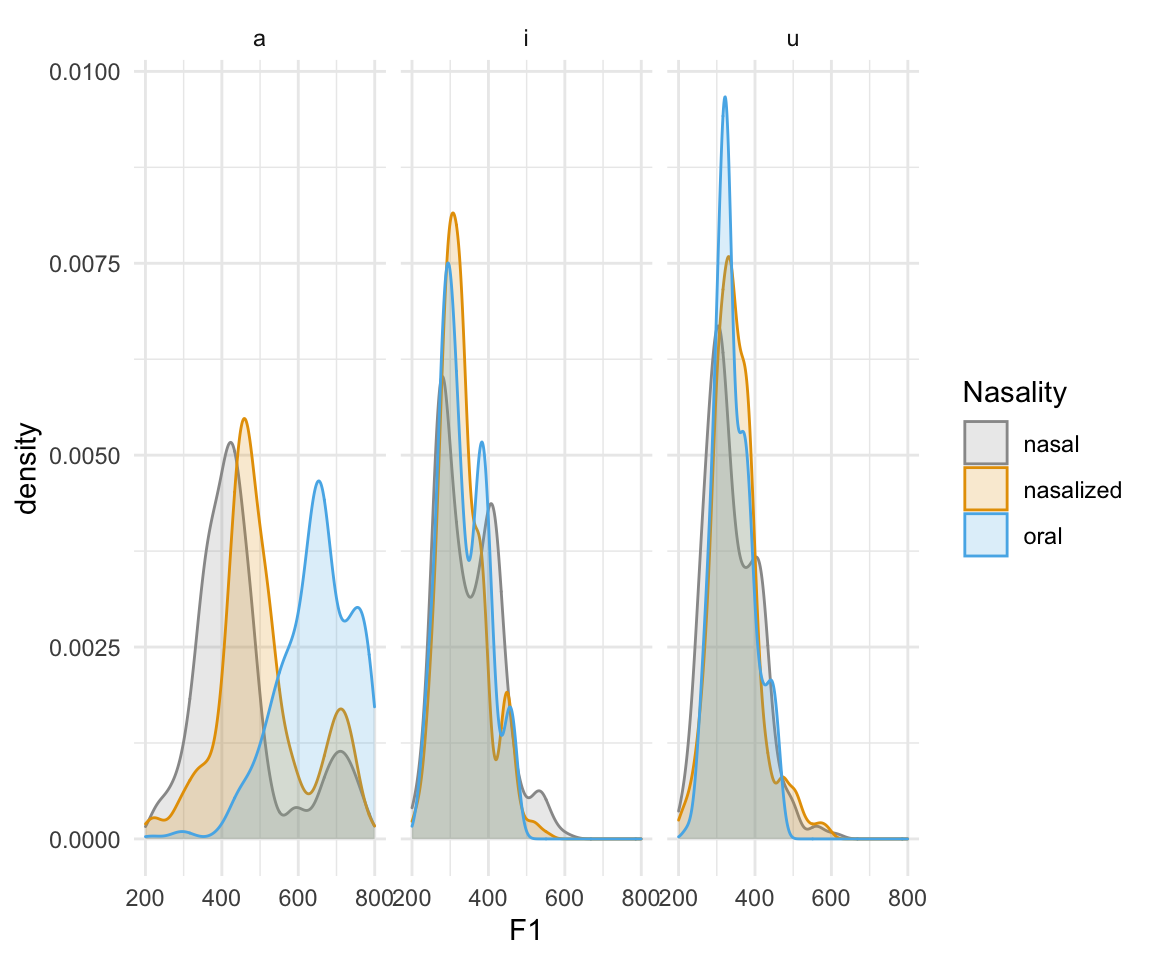

Step 2: Define the model and priors

Here, I am going to run three models for F1: one null model, one simple model, and one complex model.

Null model: F1~1 (i.e., no categorical differences) Simple model: F1~ Vowel Complex model: F1~ Vowel*Nasality + (Vowel*Nasality|Speaker)

Determining priors

The information we give the model from the past is called a prior. There are a few different types of priors, all of which are given based on reasonable ideas of what these variables can be.

For example, when we look at formant values, we have a reasonable idea of where our phonemes should lie - even including individual differences. F1 falls within about \(200-1000 Hz\) - so its mean is about \(600 Hz\), with a standard deviation of \(200 Hz\). In R we can represent this with the normal distribution. Recall that with normally distributed data, 95% of the data falls within 2 standard deviations of the mean, so we are effectively saying that we expect with 95% certainty for a value of F1 to fall in this distribution.

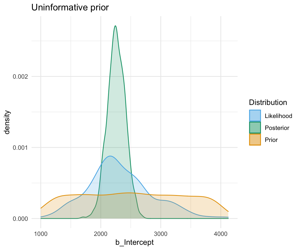
An uninformative prior is when there is no information available on the prior distribution of the model. In this case, we can consider implicitly the prior to be a uniform distribution - that is, there is an even distribution of probability for each value of RT. Graphing this (in orange below) against the original data (in blue below) gives a high weight to the data in determining the posterior probability of the model (in black below)

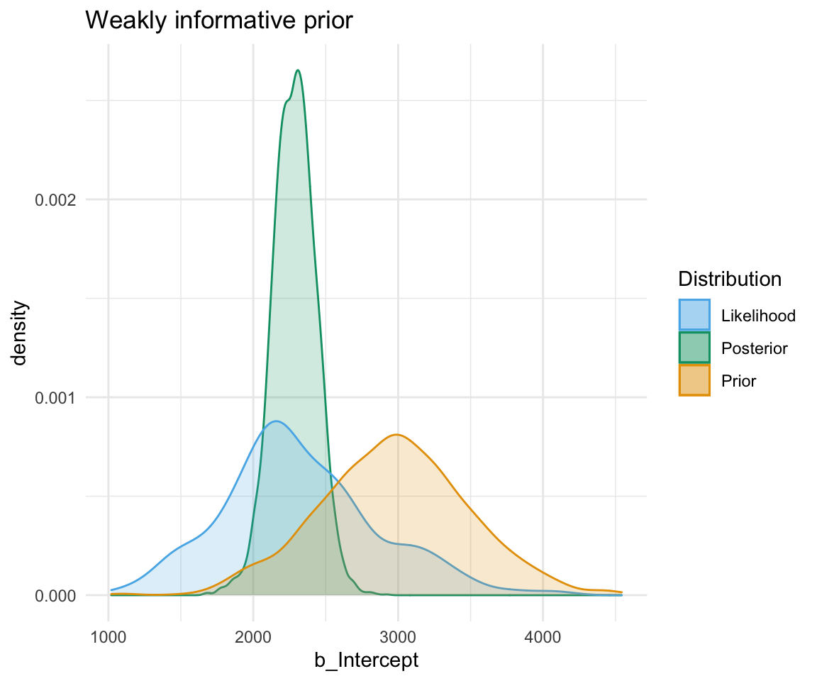
A weakly informative prior is one that helps support prior information, but still has a relatively wide distribution. In this case, the prior does somewhat affect the posterior, but its shape is still dominated by the data (aka likelihood).

To show you the effects of weakly informative priors on a model I will run a model with priors but not show you its specifications - we’ll look at the models in a bit.

A highly informative prior (or just informative prior) is one with a strong influence on the posterior. This is becase it has a much narrower range of its distribution, given a smaller standard deviation. In this case, the prior “pulls” the posterior in its direction, even though there is still the likelihood to influence the model as well.

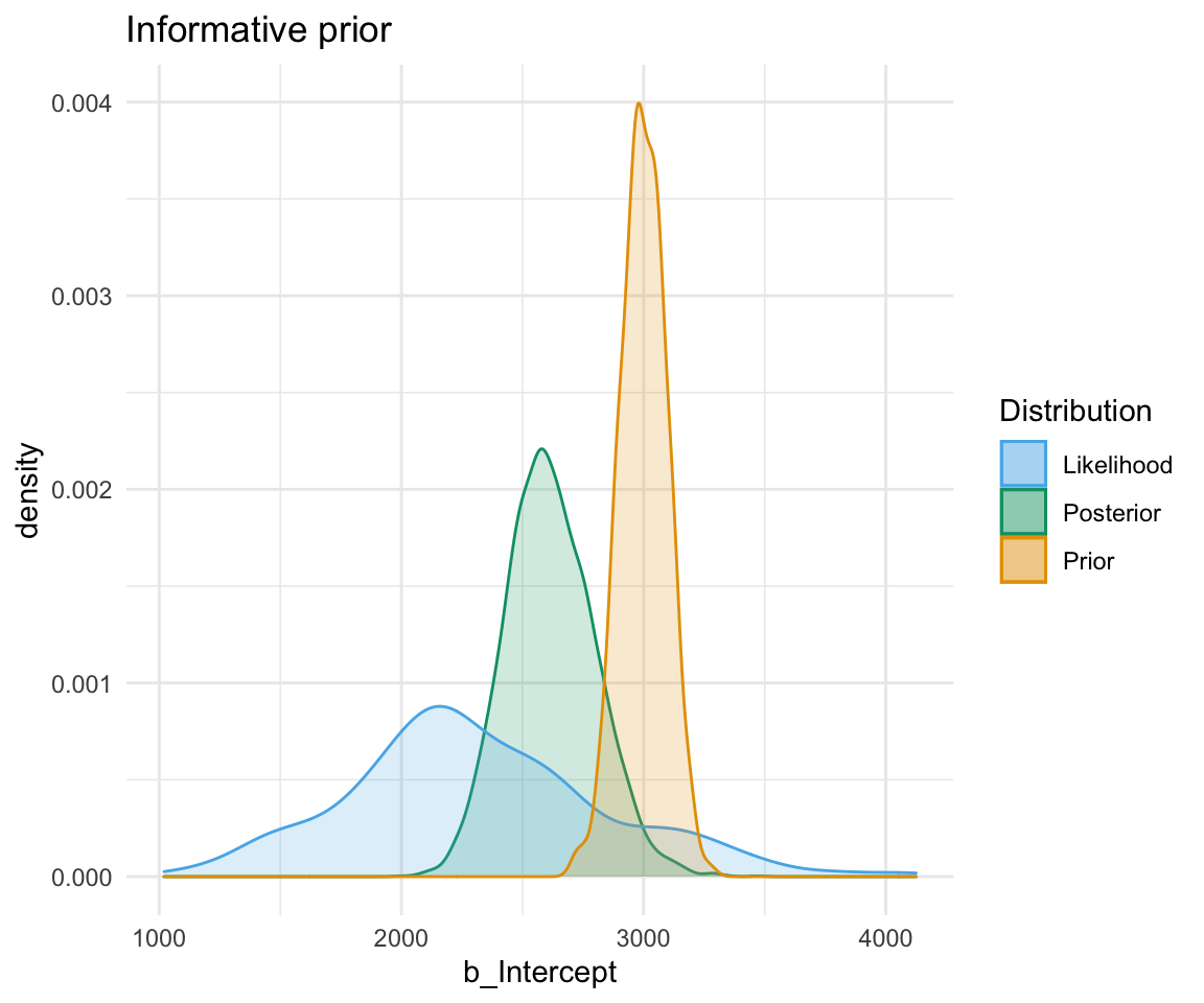
So, to directly compare these types of prior and their influence on the models:

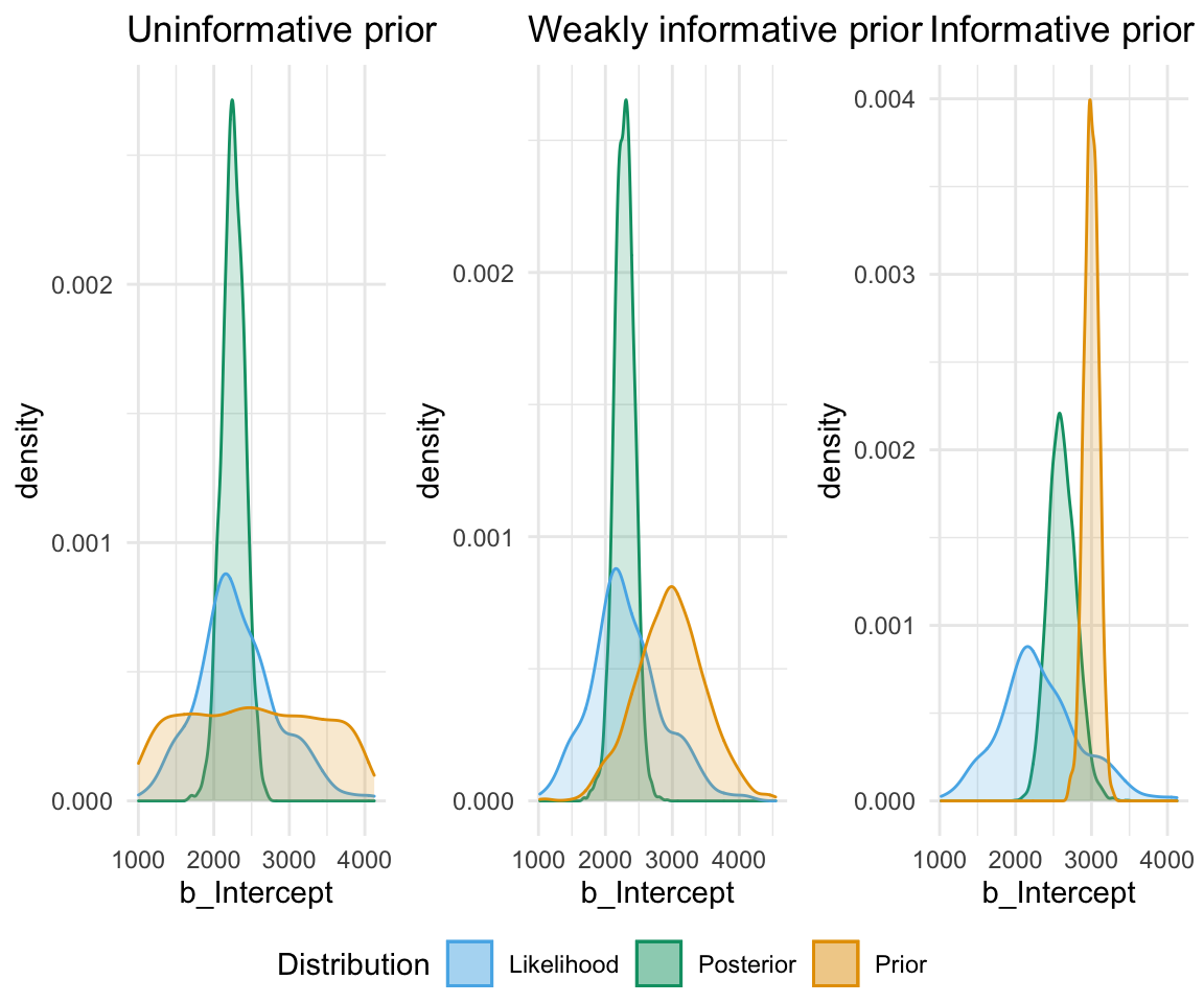
So, in short - which type of prior do we choose? Generally for continuous variables, they will have a normal distribution. We need to choose something “reasonable” - one way of doing so is pooling the literature and textbooks and deciding on a mean and standard deviation based on that. How precisely to do so still seems to be a little subjective, but if appropriate values from reputable sources are cited when making a decision, you generally should be safe.

How to set priors in brms

For each coefficient in your model, you have the option of specifying a prior. Note that when using dummy coding, we get an intercept (i.e., the baseline) and then for each level of a factor we get the “difference” estimate - how much do we expect this level to differ from the baseline? We need to specify the priors for that difference coefficient as well.

In order to get the list of priors we can specify, we can use the get_prior() function:

get_prior(F1~Nasality* Vowel + (1|Speaker), data = normtimeBP, family = gaussian())

##                     prior     class                     coef   group resp dpar
## 1                                 b                                           
## 2                                 b        Nasalitynasalized                  
## 3                                 b Nasalitynasalized:Voweli                  
## 4                                 b Nasalitynasalized:Vowelu                  
## 5                                 b             Nasalityoral                  
## 6                                 b      Nasalityoral:Voweli                  
## 7                                 b      Nasalityoral:Vowelu                  
## 8                                 b                   Voweli                  
## 9                                 b                   Vowelu                  
## 10 student_t(3, 368, 100) Intercept                                           
## 11   student_t(3, 0, 100)        sd                                           
## 12                               sd                          Speaker          
## 13                               sd                Intercept Speaker          
## 14   student_t(3, 0, 100)     sigma                                           
##    nlpar bound
## 1             
## 2             
## 3             
## 4             
## 5             
## 6             
## 7             
## 8             
## 9             
## 10            
## 11            
## 12            
## 13            
## 14

This gives the class and coefficient type for each variable. Class b (or, \(\beta\)) is a fixed effect coefficient parameter. Class sd (or, \(\sigma\)), is the standard deviation of the random effects. Class sigma is the standard deviation of the residual error. R automatically constrains sd and sigma to not have coefficients lower than 0 (since by definition standard deviations are always positive.)

To set a list of priors, we can use the set_prior() function. We need to do this for each prior we set, so it is easiest to create a list of priors and save that as a variable, then use that as the prior specification in the model.

Let’s say based on prior research we know the following with 95% certainty:

F1 ranges from 200 to 800 Hz with an average of 500 Hz.
The difference between nasal and oral vowels is anywhere from -100 to -100 Hz (average of 0 Hz), and the difference between nasal and nasalized vowels is anywhere from -50 to -50 Hz (average of 0 Hz).
The difference between a and i is around 200 to 600 Hz with an average of 400 Hz.
The difference between a and u is around 200 to 600 Hz.
Individuals can differ by 0 to 500 Hz in their F1 range.

RECALL that when we use distributions to set up our standard deviations to be half of what the difference is, since with 95% confidence we say that our values are falling within 2 standard deviations of the mean. Therefore, for reaction time (as an example), if we are pretty sure the “true value” is \(500 \pm 300\), we are saying we are 95% certain that our value falls within \(\mu \pm 2*\sigma = 500 \pm 300\), so here \(\mu = 500\) and \(2\sigma = 300\), so \(\sigma=150\).

modelpriors0 = set_prior("normal(2500,150)", class = "Intercept")

modelpriors1 = c(set_prior("normal(2500,150)", class = "Intercept"),
              set_prior("normal(400,100)", class = "b", coef = "Voweli"),
              set_prior("normal(400,100)", class = "b", coef = "Vowelu"),              
              set_prior("normal(0,250)", class = "sigma"))


modelpriors2 = c(set_prior("normal(2500,150)", class = "Intercept"),
              set_prior("normal(400,100)", class = "b", coef = "Voweli"),
              set_prior("normal(400,100)", class = "b", coef = "Vowelu"),              
              set_prior("normal(0,50)", class = "b", coef = "Nasalityoral"),
              set_prior("normal(0,25)", class = "b", coef = "Nasalitynasalized"),
              set_prior("normal(0,250)", class = "sd"),
              set_prior("normal(0,250)", class = "sigma"))

Step 3: Fit models to data

These models can take a bit of time to run, so be patient! Imagine an experimental dataset with thousands of lines. What the brm() function does is create code in Stan, which then runs in C++.

With each model, we need to define the following:

formula (same as in lme4 syntax)
dataset
family (gaussian, binomial, multinomial, etc.)
priors (more on this later!)
number of iterations sampled from the posterior distribution per chain (defaults to 2000)
number of (Markov) chains - random values are sequentially generated in each chain, where each sample depends on the previous one. Different chains are independent of each other such that running a model with four chains is equivalent to running four models with one chain each.
number of warmup iterations, which are used for settling on a posterior distribution but then are discarted (defaults to half of the number of iterations)
control (list of of parameters to control the sampler’s behavior)
- Adapt_delta: Increasing adapt_delta will slow down the sampler but will decrease the number of divergent transitions threatening the validity of your posterior samples. If you see warnings in your model about “x divergent transitions”, you should increase delta to between 0.8 and 1.

f1modelnull = brm(F1~1, data = normtimeBP, family = gaussian(), prior = modelpriors0, iter = 2000, chains = 4, warmup = 1000, control = list(adapt_delta = 0.99))

## Compiling the C++ model

## Start sampling

## 
## SAMPLING FOR MODEL '6b7dcf02f647cde107e41a9508afb413' NOW (CHAIN 1).
## Chain 1: 
## Chain 1: Gradient evaluation took 6.9e-05 seconds
## Chain 1: 1000 transitions using 10 leapfrog steps per transition would take 0.69 seconds.
## Chain 1: Adjust your expectations accordingly!
## Chain 1: 
## Chain 1: 
## Chain 1: Iteration:    1 / 2000 [  0%]  (Warmup)
## Chain 1: Iteration:  200 / 2000 [ 10%]  (Warmup)
## Chain 1: Iteration:  400 / 2000 [ 20%]  (Warmup)
## Chain 1: Iteration:  600 / 2000 [ 30%]  (Warmup)
## Chain 1: Iteration:  800 / 2000 [ 40%]  (Warmup)
## Chain 1: Iteration: 1000 / 2000 [ 50%]  (Warmup)
## Chain 1: Iteration: 1001 / 2000 [ 50%]  (Sampling)
## Chain 1: Iteration: 1200 / 2000 [ 60%]  (Sampling)
## Chain 1: Iteration: 1400 / 2000 [ 70%]  (Sampling)
## Chain 1: Iteration: 1600 / 2000 [ 80%]  (Sampling)
## Chain 1: Iteration: 1800 / 2000 [ 90%]  (Sampling)
## Chain 1: Iteration: 2000 / 2000 [100%]  (Sampling)
## Chain 1: 
## Chain 1:  Elapsed Time: 0.529783 seconds (Warm-up)
## Chain 1:                0.643061 seconds (Sampling)
## Chain 1:                1.17284 seconds (Total)
## Chain 1: 
## 
## SAMPLING FOR MODEL '6b7dcf02f647cde107e41a9508afb413' NOW (CHAIN 2).
## Chain 2: 
## Chain 2: Gradient evaluation took 5.2e-05 seconds
## Chain 2: 1000 transitions using 10 leapfrog steps per transition would take 0.52 seconds.
## Chain 2: Adjust your expectations accordingly!
## Chain 2: 
## Chain 2: 
## Chain 2: Iteration:    1 / 2000 [  0%]  (Warmup)
## Chain 2: Iteration:  200 / 2000 [ 10%]  (Warmup)
## Chain 2: Iteration:  400 / 2000 [ 20%]  (Warmup)
## Chain 2: Iteration:  600 / 2000 [ 30%]  (Warmup)
## Chain 2: Iteration:  800 / 2000 [ 40%]  (Warmup)
## Chain 2: Iteration: 1000 / 2000 [ 50%]  (Warmup)
## Chain 2: Iteration: 1001 / 2000 [ 50%]  (Sampling)
## Chain 2: Iteration: 1200 / 2000 [ 60%]  (Sampling)
## Chain 2: Iteration: 1400 / 2000 [ 70%]  (Sampling)
## Chain 2: Iteration: 1600 / 2000 [ 80%]  (Sampling)
## Chain 2: Iteration: 1800 / 2000 [ 90%]  (Sampling)
## Chain 2: Iteration: 2000 / 2000 [100%]  (Sampling)
## Chain 2: 
## Chain 2:  Elapsed Time: 0.695492 seconds (Warm-up)
## Chain 2:                0.572328 seconds (Sampling)
## Chain 2:                1.26782 seconds (Total)
## Chain 2: 
## 
## SAMPLING FOR MODEL '6b7dcf02f647cde107e41a9508afb413' NOW (CHAIN 3).
## Chain 3: 
## Chain 3: Gradient evaluation took 5e-05 seconds
## Chain 3: 1000 transitions using 10 leapfrog steps per transition would take 0.5 seconds.
## Chain 3: Adjust your expectations accordingly!
## Chain 3: 
## Chain 3: 
## Chain 3: Iteration:    1 / 2000 [  0%]  (Warmup)
## Chain 3: Iteration:  200 / 2000 [ 10%]  (Warmup)
## Chain 3: Iteration:  400 / 2000 [ 20%]  (Warmup)
## Chain 3: Iteration:  600 / 2000 [ 30%]  (Warmup)
## Chain 3: Iteration:  800 / 2000 [ 40%]  (Warmup)
## Chain 3: Iteration: 1000 / 2000 [ 50%]  (Warmup)
## Chain 3: Iteration: 1001 / 2000 [ 50%]  (Sampling)
## Chain 3: Iteration: 1200 / 2000 [ 60%]  (Sampling)
## Chain 3: Iteration: 1400 / 2000 [ 70%]  (Sampling)
## Chain 3: Iteration: 1600 / 2000 [ 80%]  (Sampling)
## Chain 3: Iteration: 1800 / 2000 [ 90%]  (Sampling)
## Chain 3: Iteration: 2000 / 2000 [100%]  (Sampling)
## Chain 3: 
## Chain 3:  Elapsed Time: 0.610774 seconds (Warm-up)
## Chain 3:                0.400948 seconds (Sampling)
## Chain 3:                1.01172 seconds (Total)
## Chain 3: 
## 
## SAMPLING FOR MODEL '6b7dcf02f647cde107e41a9508afb413' NOW (CHAIN 4).
## Chain 4: 
## Chain 4: Gradient evaluation took 5e-05 seconds
## Chain 4: 1000 transitions using 10 leapfrog steps per transition would take 0.5 seconds.
## Chain 4: Adjust your expectations accordingly!
## Chain 4: 
## Chain 4: 
## Chain 4: Iteration:    1 / 2000 [  0%]  (Warmup)
## Chain 4: Iteration:  200 / 2000 [ 10%]  (Warmup)
## Chain 4: Iteration:  400 / 2000 [ 20%]  (Warmup)
## Chain 4: Iteration:  600 / 2000 [ 30%]  (Warmup)
## Chain 4: Iteration:  800 / 2000 [ 40%]  (Warmup)
## Chain 4: Iteration: 1000 / 2000 [ 50%]  (Warmup)
## Chain 4: Iteration: 1001 / 2000 [ 50%]  (Sampling)
## Chain 4: Iteration: 1200 / 2000 [ 60%]  (Sampling)
## Chain 4: Iteration: 1400 / 2000 [ 70%]  (Sampling)
## Chain 4: Iteration: 1600 / 2000 [ 80%]  (Sampling)
## Chain 4: Iteration: 1800 / 2000 [ 90%]  (Sampling)
## Chain 4: Iteration: 2000 / 2000 [100%]  (Sampling)
## Chain 4: 
## Chain 4:  Elapsed Time: 0.611174 seconds (Warm-up)
## Chain 4:                0.414826 seconds (Sampling)
## Chain 4:                1.026 seconds (Total)
## Chain 4:

f1modelsimple = brm(F1~Vowel, data = normtimeBP,prior = modelpriors1, family = gaussian(), iter = 2000, chains = 4, warmup = 1000, control = list(adapt_delta = 0.99))

## Compiling the C++ model
## Start sampling

## 
## SAMPLING FOR MODEL '9570cab489e07418ab9f77d031d37716' NOW (CHAIN 1).
## Chain 1: 
## Chain 1: Gradient evaluation took 2.5e-05 seconds
## Chain 1: 1000 transitions using 10 leapfrog steps per transition would take 0.25 seconds.
## Chain 1: Adjust your expectations accordingly!
## Chain 1: 
## Chain 1: 
## Chain 1: Iteration:    1 / 2000 [  0%]  (Warmup)
## Chain 1: Iteration:  200 / 2000 [ 10%]  (Warmup)
## Chain 1: Iteration:  400 / 2000 [ 20%]  (Warmup)
## Chain 1: Iteration:  600 / 2000 [ 30%]  (Warmup)
## Chain 1: Iteration:  800 / 2000 [ 40%]  (Warmup)
## Chain 1: Iteration: 1000 / 2000 [ 50%]  (Warmup)
## Chain 1: Iteration: 1001 / 2000 [ 50%]  (Sampling)
## Chain 1: Iteration: 1200 / 2000 [ 60%]  (Sampling)
## Chain 1: Iteration: 1400 / 2000 [ 70%]  (Sampling)
## Chain 1: Iteration: 1600 / 2000 [ 80%]  (Sampling)
## Chain 1: Iteration: 1800 / 2000 [ 90%]  (Sampling)
## Chain 1: Iteration: 2000 / 2000 [100%]  (Sampling)
## Chain 1: 
## Chain 1:  Elapsed Time: 0.47046 seconds (Warm-up)
## Chain 1:                0.29452 seconds (Sampling)
## Chain 1:                0.76498 seconds (Total)
## Chain 1: 
## 
## SAMPLING FOR MODEL '9570cab489e07418ab9f77d031d37716' NOW (CHAIN 2).
## Chain 2: 
## Chain 2: Gradient evaluation took 1.9e-05 seconds
## Chain 2: 1000 transitions using 10 leapfrog steps per transition would take 0.19 seconds.
## Chain 2: Adjust your expectations accordingly!
## Chain 2: 
## Chain 2: 
## Chain 2: Iteration:    1 / 2000 [  0%]  (Warmup)
## Chain 2: Iteration:  200 / 2000 [ 10%]  (Warmup)
## Chain 2: Iteration:  400 / 2000 [ 20%]  (Warmup)
## Chain 2: Iteration:  600 / 2000 [ 30%]  (Warmup)
## Chain 2: Iteration:  800 / 2000 [ 40%]  (Warmup)
## Chain 2: Iteration: 1000 / 2000 [ 50%]  (Warmup)
## Chain 2: Iteration: 1001 / 2000 [ 50%]  (Sampling)
## Chain 2: Iteration: 1200 / 2000 [ 60%]  (Sampling)
## Chain 2: Iteration: 1400 / 2000 [ 70%]  (Sampling)
## Chain 2: Iteration: 1600 / 2000 [ 80%]  (Sampling)
## Chain 2: Iteration: 1800 / 2000 [ 90%]  (Sampling)
## Chain 2: Iteration: 2000 / 2000 [100%]  (Sampling)
## Chain 2: 
## Chain 2:  Elapsed Time: 0.541447 seconds (Warm-up)
## Chain 2:                0.244115 seconds (Sampling)
## Chain 2:                0.785562 seconds (Total)
## Chain 2: 
## 
## SAMPLING FOR MODEL '9570cab489e07418ab9f77d031d37716' NOW (CHAIN 3).
## Chain 3: 
## Chain 3: Gradient evaluation took 1.9e-05 seconds
## Chain 3: 1000 transitions using 10 leapfrog steps per transition would take 0.19 seconds.
## Chain 3: Adjust your expectations accordingly!
## Chain 3: 
## Chain 3: 
## Chain 3: Iteration:    1 / 2000 [  0%]  (Warmup)
## Chain 3: Iteration:  200 / 2000 [ 10%]  (Warmup)
## Chain 3: Iteration:  400 / 2000 [ 20%]  (Warmup)
## Chain 3: Iteration:  600 / 2000 [ 30%]  (Warmup)
## Chain 3: Iteration:  800 / 2000 [ 40%]  (Warmup)
## Chain 3: Iteration: 1000 / 2000 [ 50%]  (Warmup)
## Chain 3: Iteration: 1001 / 2000 [ 50%]  (Sampling)
## Chain 3: Iteration: 1200 / 2000 [ 60%]  (Sampling)
## Chain 3: Iteration: 1400 / 2000 [ 70%]  (Sampling)
## Chain 3: Iteration: 1600 / 2000 [ 80%]  (Sampling)
## Chain 3: Iteration: 1800 / 2000 [ 90%]  (Sampling)
## Chain 3: Iteration: 2000 / 2000 [100%]  (Sampling)
## Chain 3: 
## Chain 3:  Elapsed Time: 0.387194 seconds (Warm-up)
## Chain 3:                0.243468 seconds (Sampling)
## Chain 3:                0.630662 seconds (Total)
## Chain 3: 
## 
## SAMPLING FOR MODEL '9570cab489e07418ab9f77d031d37716' NOW (CHAIN 4).
## Chain 4: 
## Chain 4: Gradient evaluation took 2e-05 seconds
## Chain 4: 1000 transitions using 10 leapfrog steps per transition would take 0.2 seconds.
## Chain 4: Adjust your expectations accordingly!
## Chain 4: 
## Chain 4: 
## Chain 4: Iteration:    1 / 2000 [  0%]  (Warmup)
## Chain 4: Iteration:  200 / 2000 [ 10%]  (Warmup)
## Chain 4: Iteration:  400 / 2000 [ 20%]  (Warmup)
## Chain 4: Iteration:  600 / 2000 [ 30%]  (Warmup)
## Chain 4: Iteration:  800 / 2000 [ 40%]  (Warmup)
## Chain 4: Iteration: 1000 / 2000 [ 50%]  (Warmup)
## Chain 4: Iteration: 1001 / 2000 [ 50%]  (Sampling)
## Chain 4: Iteration: 1200 / 2000 [ 60%]  (Sampling)
## Chain 4: Iteration: 1400 / 2000 [ 70%]  (Sampling)
## Chain 4: Iteration: 1600 / 2000 [ 80%]  (Sampling)
## Chain 4: Iteration: 1800 / 2000 [ 90%]  (Sampling)
## Chain 4: Iteration: 2000 / 2000 [100%]  (Sampling)
## Chain 4: 
## Chain 4:  Elapsed Time: 0.538498 seconds (Warm-up)
## Chain 4:                0.287831 seconds (Sampling)
## Chain 4:                0.826329 seconds (Total)
## Chain 4:

f1modelcomplex = brm(F1~Nasality* Vowel + (1|Speaker), data = normtimeBP, family = gaussian(), prior = modelpriors2,  iter = 2000, chains = 4, warmup = 1000, control = list(adapt_delta = 0.99))

## Compiling the C++ model
## Start sampling

## 
## SAMPLING FOR MODEL 'f17b1ba92cdbff8d0ba076d193397cb7' NOW (CHAIN 1).
## Chain 1: 
## Chain 1: Gradient evaluation took 0.000596 seconds
## Chain 1: 1000 transitions using 10 leapfrog steps per transition would take 5.96 seconds.
## Chain 1: Adjust your expectations accordingly!
## Chain 1: 
## Chain 1: 
## Chain 1: Iteration:    1 / 2000 [  0%]  (Warmup)
## Chain 1: Iteration:  200 / 2000 [ 10%]  (Warmup)
## Chain 1: Iteration:  400 / 2000 [ 20%]  (Warmup)
## Chain 1: Iteration:  600 / 2000 [ 30%]  (Warmup)
## Chain 1: Iteration:  800 / 2000 [ 40%]  (Warmup)
## Chain 1: Iteration: 1000 / 2000 [ 50%]  (Warmup)
## Chain 1: Iteration: 1001 / 2000 [ 50%]  (Sampling)
## Chain 1: Iteration: 1200 / 2000 [ 60%]  (Sampling)
## Chain 1: Iteration: 1400 / 2000 [ 70%]  (Sampling)
## Chain 1: Iteration: 1600 / 2000 [ 80%]  (Sampling)
## Chain 1: Iteration: 1800 / 2000 [ 90%]  (Sampling)
## Chain 1: Iteration: 2000 / 2000 [100%]  (Sampling)
## Chain 1: 
## Chain 1:  Elapsed Time: 209.311 seconds (Warm-up)
## Chain 1:                257.796 seconds (Sampling)
## Chain 1:                467.107 seconds (Total)
## Chain 1: 
## 
## SAMPLING FOR MODEL 'f17b1ba92cdbff8d0ba076d193397cb7' NOW (CHAIN 2).
## Chain 2: 
## Chain 2: Gradient evaluation took 0.000246 seconds
## Chain 2: 1000 transitions using 10 leapfrog steps per transition would take 2.46 seconds.
## Chain 2: Adjust your expectations accordingly!
## Chain 2: 
## Chain 2: 
## Chain 2: Iteration:    1 / 2000 [  0%]  (Warmup)
## Chain 2: Iteration:  200 / 2000 [ 10%]  (Warmup)
## Chain 2: Iteration:  400 / 2000 [ 20%]  (Warmup)
## Chain 2: Iteration:  600 / 2000 [ 30%]  (Warmup)
## Chain 2: Iteration:  800 / 2000 [ 40%]  (Warmup)
## Chain 2: Iteration: 1000 / 2000 [ 50%]  (Warmup)
## Chain 2: Iteration: 1001 / 2000 [ 50%]  (Sampling)
## Chain 2: Iteration: 1200 / 2000 [ 60%]  (Sampling)
## Chain 2: Iteration: 1400 / 2000 [ 70%]  (Sampling)
## Chain 2: Iteration: 1600 / 2000 [ 80%]  (Sampling)
## Chain 2: Iteration: 1800 / 2000 [ 90%]  (Sampling)
## Chain 2: Iteration: 2000 / 2000 [100%]  (Sampling)
## Chain 2: 
## Chain 2:  Elapsed Time: 218.323 seconds (Warm-up)
## Chain 2:                245.731 seconds (Sampling)
## Chain 2:                464.054 seconds (Total)
## Chain 2: 
## 
## SAMPLING FOR MODEL 'f17b1ba92cdbff8d0ba076d193397cb7' NOW (CHAIN 3).
## Chain 3: 
## Chain 3: Gradient evaluation took 0.000247 seconds
## Chain 3: 1000 transitions using 10 leapfrog steps per transition would take 2.47 seconds.
## Chain 3: Adjust your expectations accordingly!
## Chain 3: 
## Chain 3: 
## Chain 3: Iteration:    1 / 2000 [  0%]  (Warmup)
## Chain 3: Iteration:  200 / 2000 [ 10%]  (Warmup)
## Chain 3: Iteration:  400 / 2000 [ 20%]  (Warmup)
## Chain 3: Iteration:  600 / 2000 [ 30%]  (Warmup)
## Chain 3: Iteration:  800 / 2000 [ 40%]  (Warmup)
## Chain 3: Iteration: 1000 / 2000 [ 50%]  (Warmup)
## Chain 3: Iteration: 1001 / 2000 [ 50%]  (Sampling)
## Chain 3: Iteration: 1200 / 2000 [ 60%]  (Sampling)
## Chain 3: Iteration: 1400 / 2000 [ 70%]  (Sampling)
## Chain 3: Iteration: 1600 / 2000 [ 80%]  (Sampling)
## Chain 3: Iteration: 1800 / 2000 [ 90%]  (Sampling)
## Chain 3: Iteration: 2000 / 2000 [100%]  (Sampling)
## Chain 3: 
## Chain 3:  Elapsed Time: 217.101 seconds (Warm-up)
## Chain 3:                250.19 seconds (Sampling)
## Chain 3:                467.291 seconds (Total)
## Chain 3: 
## 
## SAMPLING FOR MODEL 'f17b1ba92cdbff8d0ba076d193397cb7' NOW (CHAIN 4).
## Chain 4: 
## Chain 4: Gradient evaluation took 0.000265 seconds
## Chain 4: 1000 transitions using 10 leapfrog steps per transition would take 2.65 seconds.
## Chain 4: Adjust your expectations accordingly!
## Chain 4: 
## Chain 4: 
## Chain 4: Iteration:    1 / 2000 [  0%]  (Warmup)
## Chain 4: Iteration:  200 / 2000 [ 10%]  (Warmup)
## Chain 4: Iteration:  400 / 2000 [ 20%]  (Warmup)
## Chain 4: Iteration:  600 / 2000 [ 30%]  (Warmup)
## Chain 4: Iteration:  800 / 2000 [ 40%]  (Warmup)
## Chain 4: Iteration: 1000 / 2000 [ 50%]  (Warmup)
## Chain 4: Iteration: 1001 / 2000 [ 50%]  (Sampling)
## Chain 4: Iteration: 1200 / 2000 [ 60%]  (Sampling)
## Chain 4: Iteration: 1400 / 2000 [ 70%]  (Sampling)
## Chain 4: Iteration: 1600 / 2000 [ 80%]  (Sampling)
## Chain 4: Iteration: 1800 / 2000 [ 90%]  (Sampling)
## Chain 4: Iteration: 2000 / 2000 [100%]  (Sampling)
## Chain 4: 
## Chain 4:  Elapsed Time: 213.968 seconds (Warm-up)
## Chain 4:                242.756 seconds (Sampling)
## Chain 4:                456.724 seconds (Total)
## Chain 4:

## Warning: There were 3676 transitions after warmup that exceeded the maximum treedepth. Increase max_treedepth above 10. See
## http://mc-stan.org/misc/warnings.html#maximum-treedepth-exceeded

## Warning: Examine the pairs() plot to diagnose sampling problems

## Warning: The largest R-hat is 1.07, indicating chains have not mixed.
## Running the chains for more iterations may help. See
## http://mc-stan.org/misc/warnings.html#r-hat

## Warning: Bulk Effective Samples Size (ESS) is too low, indicating posterior means and medians may be unreliable.
## Running the chains for more iterations may help. See
## http://mc-stan.org/misc/warnings.html#bulk-ess

## Warning: Tail Effective Samples Size (ESS) is too low, indicating posterior variances and tail quantiles may be unreliable.
## Running the chains for more iterations may help. See
## http://mc-stan.org/misc/warnings.html#tail-ess

Step 4: Check model convergence

Like with frequentist mixed effects models, it is important to check whether or not a model has converged. One metric for convergence is the \(\widehat{R}\) (R-hat) statistic, which is the ratio of between-chain to within-chain variance. We expect the \(\widehat{R}\) to be around 1, meaning there is a comparable amount of within-chain and between-chain variance.

To get the \(\widehat{R}\) value, use summary to look at the model. You can also plot the \(\widehat{R}\) values for each parameter using the mcmc_rhat() function from the bayesplot package.

summary(f1modelnull)

##  Family: gaussian 
##   Links: mu = identity; sigma = identity 
## Formula: F1 ~ 1 
##    Data: normtimeBP (Number of observations: 4655) 
## Samples: 4 chains, each with iter = 2000; warmup = 1000; thin = 1;
##          total post-warmup samples = 4000
## 
## Population-Level Effects: 
##           Estimate Est.Error l-95% CI u-95% CI Rhat Bulk_ESS Tail_ESS
## Intercept   399.88      1.92   396.10   403.78 1.00     2087     2010
## 
## Family Specific Parameters: 
##       Estimate Est.Error l-95% CI u-95% CI Rhat Bulk_ESS Tail_ESS
## sigma   128.33      1.32   125.80   130.86 1.00     2498     2090
## 
## Samples were drawn using sampling(NUTS). For each parameter, Bulk_ESS
## and Tail_ESS are effective sample size measures, and Rhat is the potential
## scale reduction factor on split chains (at convergence, Rhat = 1).

mcmc_rhat(rhat(f1modelnull))+ yaxis_text(hjust = 1)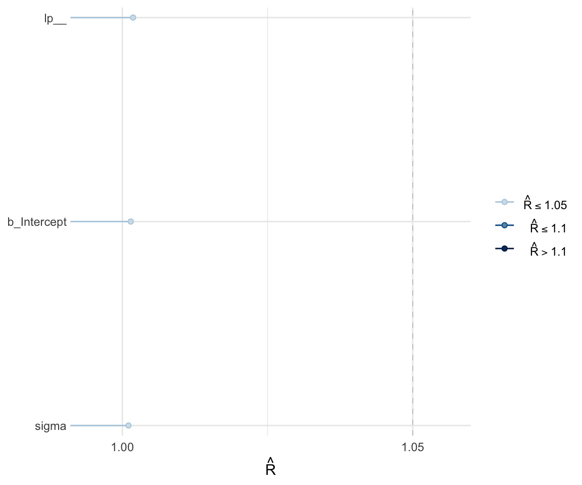

summary(f1modelsimple)

##  Family: gaussian 
##   Links: mu = identity; sigma = identity 
## Formula: F1 ~ Vowel 
##    Data: normtimeBP (Number of observations: 4655) 
## Samples: 4 chains, each with iter = 2000; warmup = 1000; thin = 1;
##          total post-warmup samples = 4000
## 
## Population-Level Effects: 
##           Estimate Est.Error l-95% CI u-95% CI Rhat Bulk_ESS Tail_ESS
## Intercept   524.52      2.45   519.67   529.34 1.00     2569     2374
## Voweli     -186.22      3.40  -192.86  -179.46 1.00     2659     2477
## Vowelu     -180.87      3.41  -187.53  -174.08 1.00     2782     2688
## 
## Family Specific Parameters: 
##       Estimate Est.Error l-95% CI u-95% CI Rhat Bulk_ESS Tail_ESS
## sigma    95.16      0.95    93.33    97.09 1.00     3848     2491
## 
## Samples were drawn using sampling(NUTS). For each parameter, Bulk_ESS
## and Tail_ESS are effective sample size measures, and Rhat is the potential
## scale reduction factor on split chains (at convergence, Rhat = 1).

mcmc_rhat(rhat(f1modelsimple))+ yaxis_text(hjust = 1)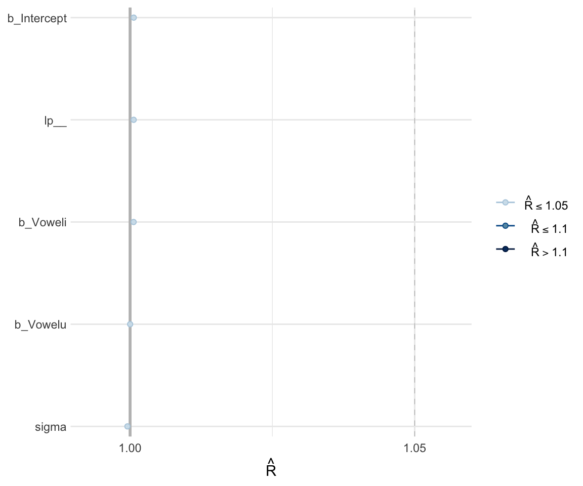

summary(f1modelcomplex)

## Warning: Parts of the model have not converged (some Rhats are > 1.05). Be
## careful when analysing the results! We recommend running more iterations and/or
## setting stronger priors.

##  Family: gaussian 
##   Links: mu = identity; sigma = identity 
## Formula: F1 ~ Nasality * Vowel + (1 | Speaker) 
##    Data: normtimeBP (Number of observations: 4655) 
## Samples: 4 chains, each with iter = 2000; warmup = 1000; thin = 1;
##          total post-warmup samples = 4000
## 
## Group-Level Effects: 
## ~Speaker (Number of levels: 12) 
##               Estimate Est.Error l-95% CI u-95% CI Rhat Bulk_ESS Tail_ESS
## sd(Intercept)  1083.28    116.68   864.27  1321.35 1.07       63      317
## 
## Population-Level Effects: 
##                          Estimate Est.Error l-95% CI u-95% CI Rhat Bulk_ESS
## Intercept                 2153.41    148.12  1868.13  2455.41 1.00      283
## Nasalitynasalized           50.93      3.97    43.35    58.86 1.02      177
## Nasalityoral               211.88      4.10   203.79   219.59 1.03      182
## Voweli                    -104.26      3.94  -112.01   -96.73 1.02      161
## Vowelu                    -111.28      3.84  -119.32  -104.07 1.04      156
## Nasalitynasalized:Voweli   -63.49      5.67   -75.31   -52.84 1.02      188
## Nasalityoral:Voweli       -222.06      5.80  -233.20  -210.06 1.03      165
## Nasalitynasalized:Vowelu   -40.25      5.66   -51.03   -29.08 1.03      167
## Nasalityoral:Vowelu       -207.81      5.71  -218.16  -196.21 1.05      130
##                          Tail_ESS
## Intercept                     782
## Nasalitynasalized             502
## Nasalityoral                  541
## Voweli                        294
## Vowelu                        262
## Nasalitynasalized:Voweli      624
## Nasalityoral:Voweli           519
## Nasalitynasalized:Vowelu      325
## Nasalityoral:Vowelu           324
## 
## Family Specific Parameters: 
##       Estimate Est.Error l-95% CI u-95% CI Rhat Bulk_ESS Tail_ESS
## sigma    65.10      0.70    63.76    66.57 1.01      504      949
## 
## Samples were drawn using sampling(NUTS). For each parameter, Bulk_ESS
## and Tail_ESS are effective sample size measures, and Rhat is the potential
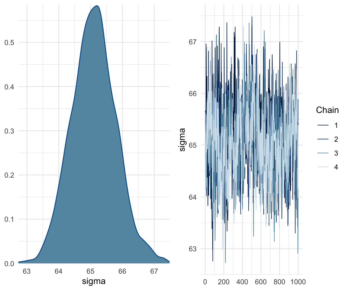
## scale reduction factor on split chains (at convergence, Rhat = 1).

mcmc_rhat(rhat(f1modelcomplex))+ yaxis_text(hjust = 1)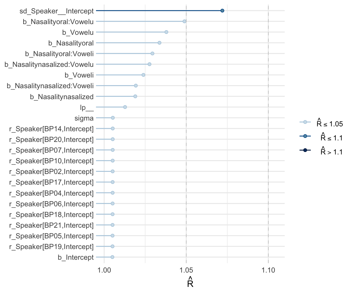

In addition, we can look at the chains - when they are plotted, they should overlap and not deviate from one another wildly. This indicates that the chains are doing more or less the same thing. We can plot the chains using the stanplot() function from brms, or the ggs_traceplot() function from ggmcmc.

plot(f1modelnull)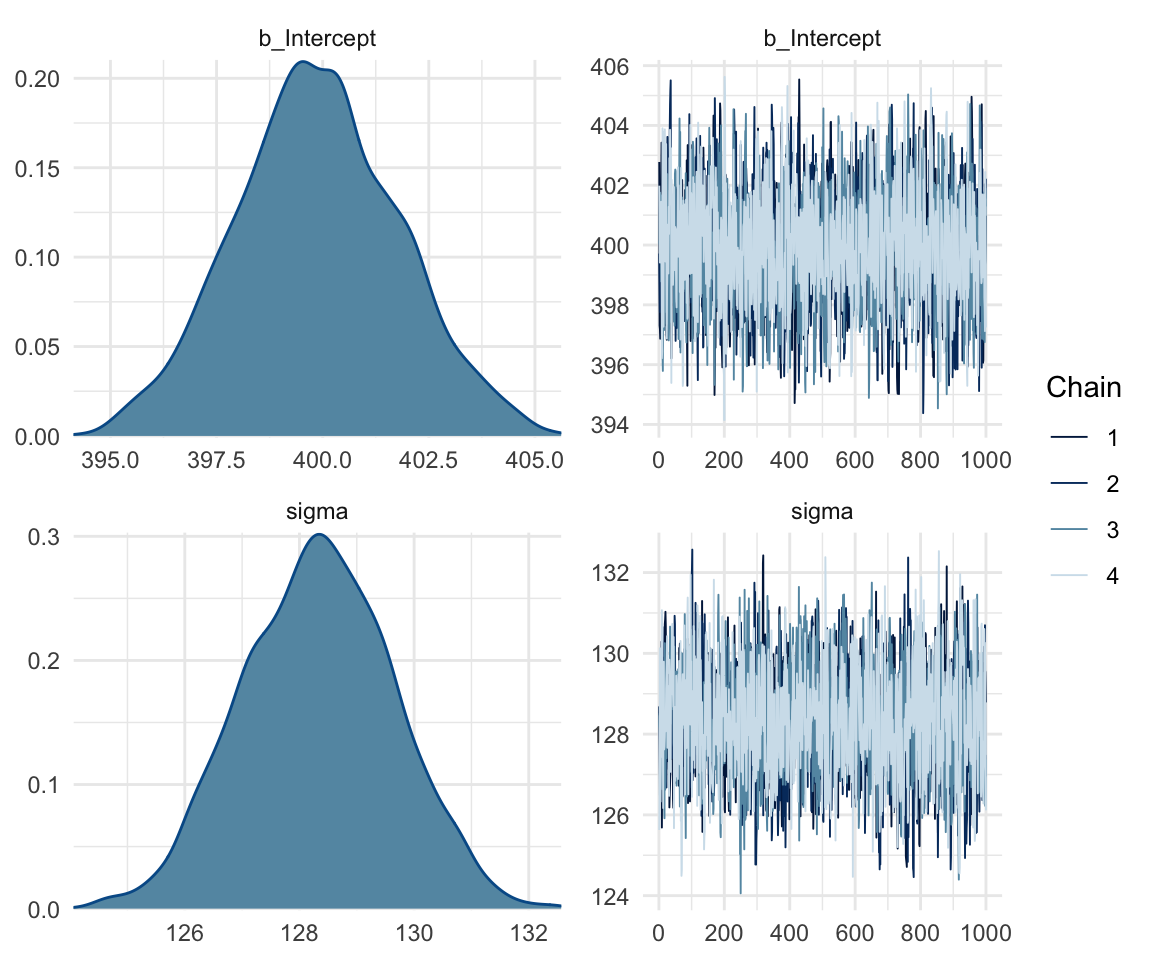

plot(f1modelsimple)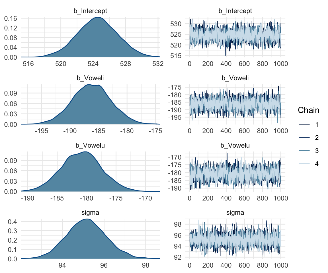

plot(f1modelcomplex)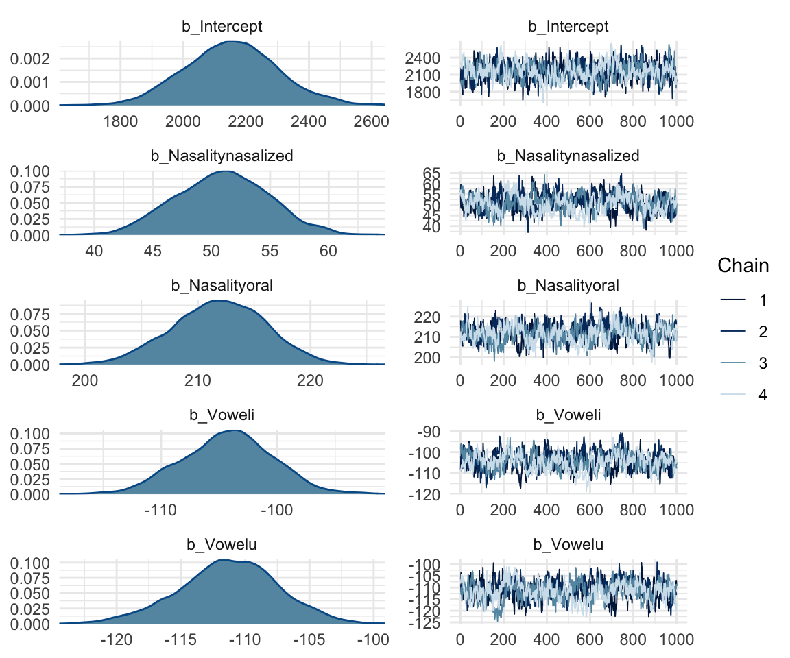

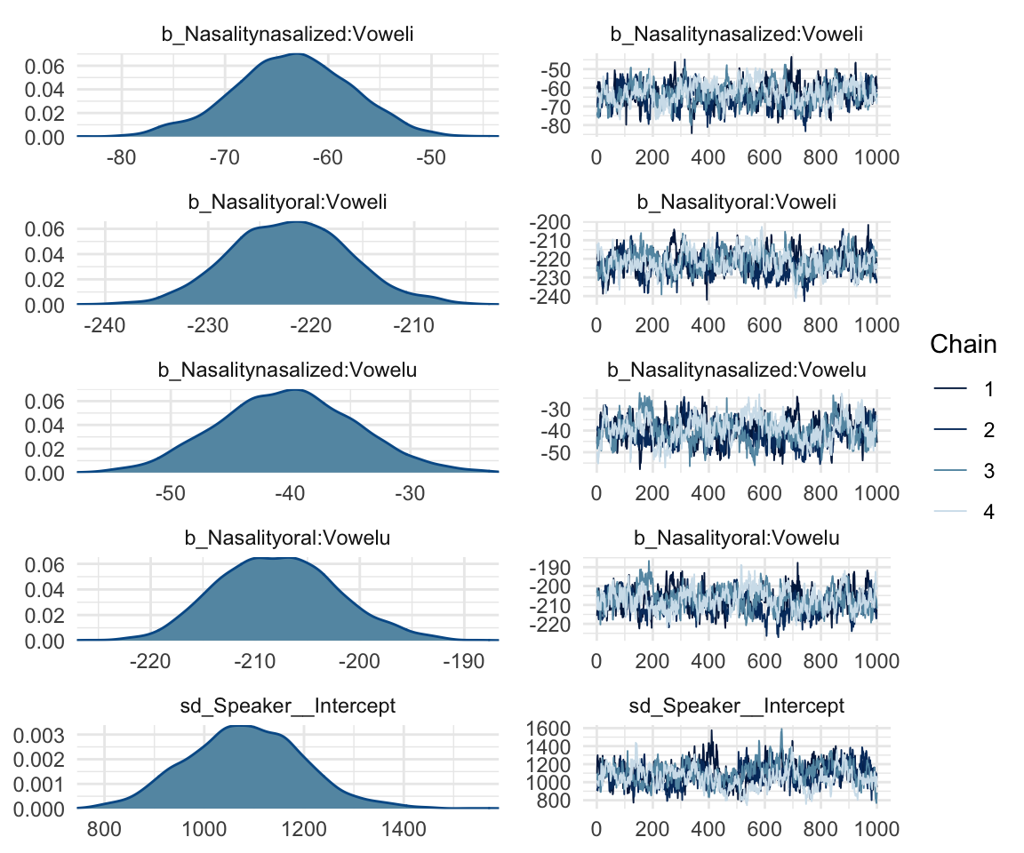
ggs_traceplot(ggs(f1modelcomplex))+ scale_color_manual(values = cbPalette)

## Warning in custom.sort(D$Parameter): NAs introduced by coercion

## Warning in custom.sort(D$Parameter): NAs introduced by coercion

## Warning: `tbl_df()` is deprecated as of dplyr 1.0.0.
## Please use `tibble::as_tibble()` instead.
## This warning is displayed once every 8 hours.
## Call `lifecycle::last_warnings()` to see where this warning was generated.

## Scale for 'colour' is already present. Adding another scale for 'colour',
## which will replace the existing scale.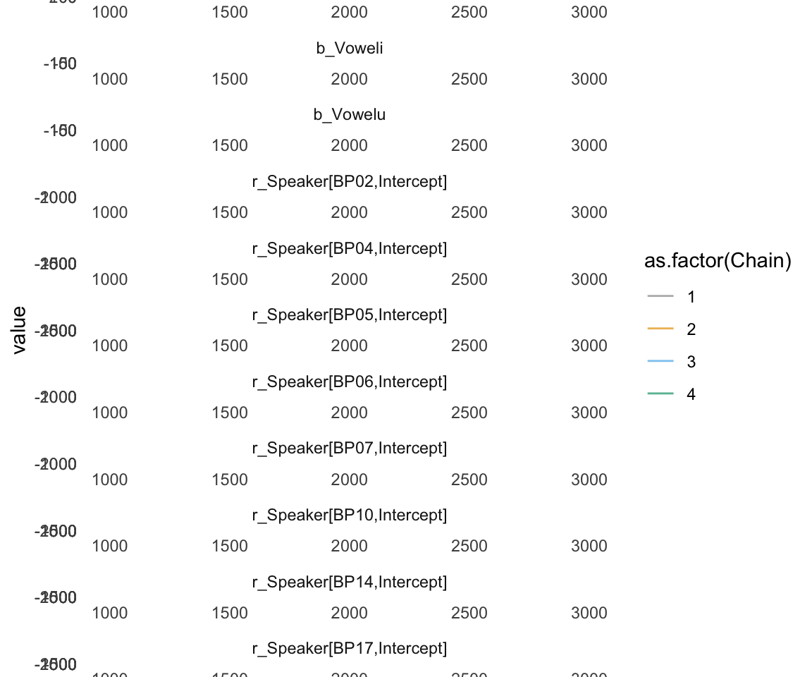

#here I am only lookng for the fixed effects parameters, or beta parameters. Otherwise we would end up with plots for every participant's intercept.

ggsf1modelcomplex = ggs(f1modelcomplex) %>% dplyr::filter(str_detect(Parameter, "^b"))

## Warning in custom.sort(D$Parameter): NAs introduced by coercion

## Warning in custom.sort(D$Parameter): NAs introduced by coercion

ggs_traceplot(ggsf1modelcomplex, original_burnin = FALSE)+ scale_color_manual(values = cbPalette)  + xlim(c(1000,2000)) + ggtitle("Model 4")

## Scale for 'colour' is already present. Adding another scale for 'colour',
## which will replace the existing scale.

## Scale for 'x' is already present. Adding another scale for 'x', which will
## replace the existing scale.

## Warning: Removed 3996 row(s) containing missing values (geom_path).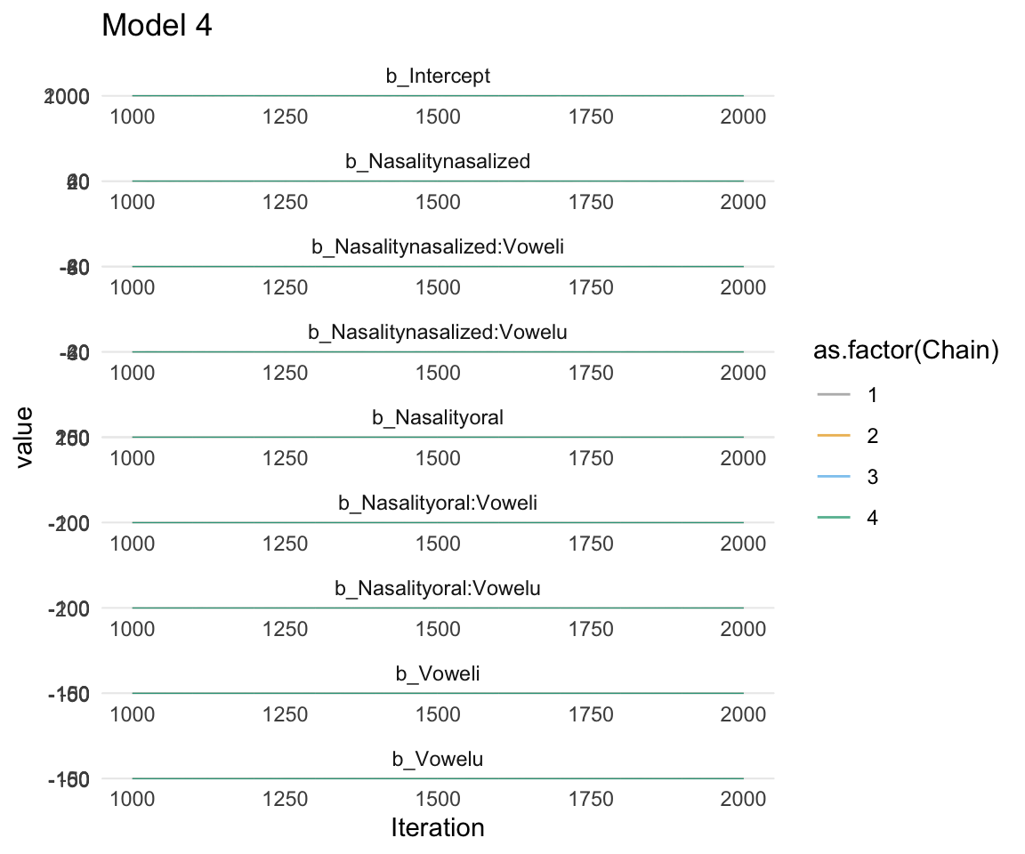

Step 5: Carry out inference

I’m going to take this a little out of order and first do some model comparison, then plot posterior distributions and do some hypothesis testing.

Evaluate predictive performance of competing models

Like with linear mixed effects models and many other analytical methods we have talked about, we need to make sure our model is fit well to our data.

There are a few different methods for doing model comparison. The first is whether your model fits the data. You can use the pp_check() function, which plots your model’s prediction against nsamples random samples, as below:

pp_check(f1modelcomplex, nsamples = 100)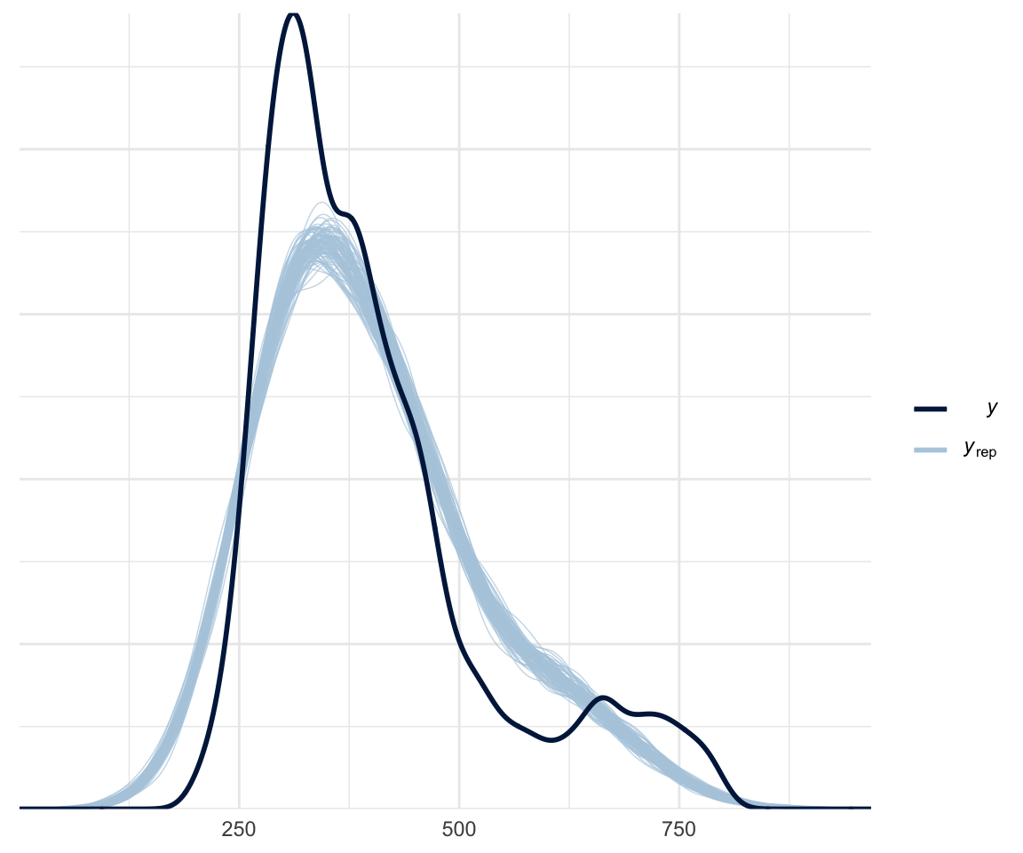

Of course, this is a bit biased, since we are plotting our data against a model which was built on said data.

A better way of looking at the model is to look at the predictive power of the model against either new data or a subset of “held-out” data. One method of this is called leave-one-out (LOO) validation. In this method (similar to cross-validation), you leave out a data point, run the model, use the model to predict that data point, and calculate the difference between the predicted and actual value. We can then compare the loo value between different models, with the model having a lower loo value considered to have the better performance.

The brms package has a built-in function, loo(), which can be used to calculate this value. The output of interest for this model is the LOOIC value.

brms::loo(f1modelnull)

## 
## Computed from 4000 by 4655 log-likelihood matrix
## 
##          Estimate    SE
## elpd_loo -29206.4  59.3
## p_loo         2.5   0.1
## looic     58412.9 118.6
## ------
## Monte Carlo SE of elpd_loo is 0.0.
## 
## All Pareto k estimates are good (k < 0.5).
## See help('pareto-k-diagnostic') for details.

In order to compare multiple models, you used to be able to include multiple into the model and say compare = TRUE, but this seems to be deprecated and doesn’t show you \(\Delta\)LOOIC values.

brms::loo(f1modelnull, f1modelsimple, f1modelcomplex, compare = T)

## Output of model 'f1modelnull':
## 
## Computed from 4000 by 4655 log-likelihood matrix
## 
##          Estimate    SE
## elpd_loo -29206.4  59.3
## p_loo         2.5   0.1
## looic     58412.9 118.6
## ------
## Monte Carlo SE of elpd_loo is 0.0.
## 
## All Pareto k estimates are good (k < 0.5).
## See help('pareto-k-diagnostic') for details.
## 
## Output of model 'f1modelsimple':
## 
## Computed from 4000 by 4655 log-likelihood matrix
## 
##          Estimate    SE
## elpd_loo -27812.2  55.2
## p_loo         4.2   0.1
## looic     55624.4 110.4
## ------
## Monte Carlo SE of elpd_loo is 0.0.
## 
## All Pareto k estimates are good (k < 0.5).
## See help('pareto-k-diagnostic') for details.
## 
## Output of model 'f1modelcomplex':
## 
## Computed from 4000 by 4655 log-likelihood matrix
## 
##          Estimate    SE
## elpd_loo -26055.5  75.2
## p_loo        23.7   1.0
## looic     52111.0 150.5
## ------
## Monte Carlo SE of elpd_loo is 0.2.
## 
## All Pareto k estimates are good (k < 0.5).
## See help('pareto-k-diagnostic') for details.
## 
## Model comparisons:
##                elpd_diff se_diff
## f1modelcomplex     0.0       0.0
## f1modelsimple  -1756.7      64.2
## f1modelnull    -3151.0      80.3

Another method we can use is to we can add the loo comparison criteria to each model (it doesn’t change the model itself!) and use loo_compare(). Unfortunately, this doesn’t seem to give \(\Delta\)LOOIC values either - but it does give ELPD-loo (expected log pointwise predictive density) differences. In this case, the model at the top “wins”, as when elpd_diff is positive then the expected predictive accuracy for the second model is higher. A negative elpd_diff favors the first model.

f1modelnull = add_criterion(f1modelnull, "loo")
f1modelsimple = add_criterion(f1modelsimple, "loo")
f1modelcomplex = add_criterion(f1modelcomplex, "loo")

loo_compare(f1modelnull, f1modelsimple, f1modelcomplex, criterion = "loo")

##                elpd_diff se_diff
## f1modelcomplex     0.0       0.0
## f1modelsimple  -1756.7      64.2
## f1modelnull    -3151.0      80.3

Other methods include Watanabe-Akaike information criterion (WAIC), kfold, marginal likelihood and R². WE can add these validation criteria to the models simultaneously. Once again,a negative elpd_diff favors the first model.

Note we cannot use loo_compare to compare R² values - we need to extract those manually. Note that while this is technically possible to do, Bayesian analyses often do not include R² in their writeups (see this conversation.)

f1modelnull = add_criterion(f1modelnull, c("R2", "waic"))

## Warning: Criterion 'R2' is deprecated. Please use 'bayes_R2' instead.

f1modelsimple = add_criterion(f1modelsimple, c("R2", "waic"))

## Warning: Criterion 'R2' is deprecated. Please use 'bayes_R2' instead.

f1modelcomplex = add_criterion(f1modelcomplex, c("R2", "waic"))

## Warning: Criterion 'R2' is deprecated. Please use 'bayes_R2' instead.

loo_compare(f1modelnull, f1modelsimple, f1modelcomplex,  criterion = "waic")

##                elpd_diff se_diff
## f1modelcomplex     0.0       0.0
## f1modelsimple  -1756.7      64.2
## f1modelnull    -3151.0      80.3

loo_compare(f1modelnull, f1modelsimple, f1modelcomplex,  criterion = "R2")

## Error in match.arg(criterion): 'arg' should be one of "loo", "waic", "kfold"

sapply(list(f1modelnull, f1modelsimple, f1modelcomplex), function(x) median(x$R2))

## [[1]]
## NULL
## 
## [[2]]
## NULL
## 
## [[3]]
## NULL

sapply(list(f1modelnull, f1modelsimple, f1modelcomplex), function(x) round(median(x$R2)*100, 2))

## [[1]]
## numeric(0)
## 
## [[2]]
## numeric(0)
## 
## [[3]]
## numeric(0)

In all of these cases, our most complex model, f1modelcomplex, is favored.

Summarize and display posterior distributions

Now that we have a model and we know it converged, how do we interpret it?

There are a few different ways of interpreting a model. The first, and most common, is to both plot and report the posterior distributions. When I say plot, I mean we literally plot the distribution, usually with a histogram. When I say report the posterior distributions, I mean plot the estimate of each parameter (aka the mode of the density plot), along with the 95% credible interval (abbreviated as CrI, rather than CI).

First, to get the posterior distributions, we use summary() from base R and posterior_summary() from brms.

summary(f1modelcomplex)

## Warning: Parts of the model have not converged (some Rhats are > 1.05). Be
## careful when analysing the results! We recommend running more iterations and/or
## setting stronger priors.

##  Family: gaussian 
##   Links: mu = identity; sigma = identity 
## Formula: F1 ~ Nasality * Vowel + (1 | Speaker) 
##    Data: normtimeBP (Number of observations: 4655) 
## Samples: 4 chains, each with iter = 2000; warmup = 1000; thin = 1;
##          total post-warmup samples = 4000
## 
## Group-Level Effects: 
## ~Speaker (Number of levels: 12) 
##               Estimate Est.Error l-95% CI u-95% CI Rhat Bulk_ESS Tail_ESS
## sd(Intercept)  1083.28    116.68   864.27  1321.35 1.07       63      317
## 
## Population-Level Effects: 
##                          Estimate Est.Error l-95% CI u-95% CI Rhat Bulk_ESS
## Intercept                 2153.41    148.12  1868.13  2455.41 1.00      283
## Nasalitynasalized           50.93      3.97    43.35    58.86 1.02      177
## Nasalityoral               211.88      4.10   203.79   219.59 1.03      182
## Voweli                    -104.26      3.94  -112.01   -96.73 1.02      161
## Vowelu                    -111.28      3.84  -119.32  -104.07 1.04      156
## Nasalitynasalized:Voweli   -63.49      5.67   -75.31   -52.84 1.02      188
## Nasalityoral:Voweli       -222.06      5.80  -233.20  -210.06 1.03      165
## Nasalitynasalized:Vowelu   -40.25      5.66   -51.03   -29.08 1.03      167
## Nasalityoral:Vowelu       -207.81      5.71  -218.16  -196.21 1.05      130
##                          Tail_ESS
## Intercept                     782
## Nasalitynasalized             502
## Nasalityoral                  541
## Voweli                        294
## Vowelu                        262
## Nasalitynasalized:Voweli      624
## Nasalityoral:Voweli           519
## Nasalitynasalized:Vowelu      325
## Nasalityoral:Vowelu           324
## 
## Family Specific Parameters: 
##       Estimate Est.Error l-95% CI u-95% CI Rhat Bulk_ESS Tail_ESS
## sigma    65.10      0.70    63.76    66.57 1.01      504      949
## 
## Samples were drawn using sampling(NUTS). For each parameter, Bulk_ESS
## and Tail_ESS are effective sample size measures, and Rhat is the potential
## scale reduction factor on split chains (at convergence, Rhat = 1).

Note that here, we get similar results to a lme4 model in terms of estimate, except we also get the 95% CrI. These are known as the \(\beta\) (or b_) coefficients, as they are changes in the fixed effects. For the mixed effects model, we are given the standard deviation for any group-level effects, meaning the varying intercept for subject. If we had included a random slope as well, we would get that sd also.

posterior_summary(f1modelcomplex)

##                                Estimate   Est.Error         Q2.5        Q97.5
## b_Intercept                  2153.41155 148.1173024   1868.13001   2455.41256
## b_Nasalitynasalized            50.93425   3.9732706     43.34835     58.86375
## b_Nasalityoral                211.87510   4.1039767    203.79385    219.58893
## b_Voweli                     -104.25611   3.9380220   -112.01409    -96.72973
## b_Vowelu                     -111.28066   3.8403194   -119.32143   -104.07029
## b_Nasalitynasalized:Voweli    -63.48802   5.6671545    -75.31267    -52.83967
## b_Nasalityoral:Voweli        -222.05743   5.8003207   -233.19982   -210.05878
## b_Nasalitynasalized:Vowelu    -40.24645   5.6643593    -51.02810    -29.07994
## b_Nasalityoral:Vowelu        -207.81080   5.7108474   -218.16077   -196.21244
## sd_Speaker__Intercept        1083.27593 116.6822902    864.27356   1321.34940
## sigma                          65.10084   0.6995072     63.76068     66.56675
## r_Speaker[BP02,Intercept]   -1715.14292 148.2232729  -2018.48105  -1433.66773
## r_Speaker[BP04,Intercept]   -1735.15296 148.2746493  -2037.51348  -1452.22254
## r_Speaker[BP05,Intercept]   -1761.29357 148.2487198  -2065.59114  -1478.45290
## r_Speaker[BP06,Intercept]   -1759.76345 148.2101623  -2061.33097  -1476.00718
## r_Speaker[BP07,Intercept]   -1680.50978 148.2429723  -1982.69333  -1396.38984
## r_Speaker[BP10,Intercept]   -1731.13629 148.3097315  -2034.68753  -1447.11622
## r_Speaker[BP14,Intercept]   -1756.92660 148.2915959  -2058.84001  -1471.61129
## r_Speaker[BP17,Intercept]   -1683.46135 148.2971795  -1986.61921  -1397.61356
## r_Speaker[BP18,Intercept]   -1691.68505 148.2250169  -1994.87118  -1409.10091
## r_Speaker[BP19,Intercept]   -1676.72877 148.3404551  -1979.59427  -1393.14374
## r_Speaker[BP20,Intercept]   -1614.73609 148.2620248  -1918.01236  -1330.16615
## r_Speaker[BP21,Intercept]   -1596.79766 148.2473929  -1897.73069  -1311.63348
## lp__                       -26146.34047   3.7118996 -26154.42795 -26140.02229

Here, we get the estimate, error, and 95% CrI for each of the beta coefficients, the sd of the random effect, the deviation for each level of the random effect, and sigma (which is the standard deviation of the residual error, and is automatically bounded to be a positive value by brms).

To plot the results, we can use stanplot() from brms, and create a histogram or interval plot, or we can use the tidybayes function add_fitted_draws() to create interval plots. We can also use the brms function marginal_effects().There are a number of other ways to do this, but these are (IMHO) the most straight forward.

stanplot(f1modelcomplex, pars = c("^b","sd","sigma"), type="hist")

## Warning: Method 'stanplot' is deprecated. Please use 'mcmc_plot' instead.

## `stat_bin()` using `bins = 30`. Pick better value with `binwidth`.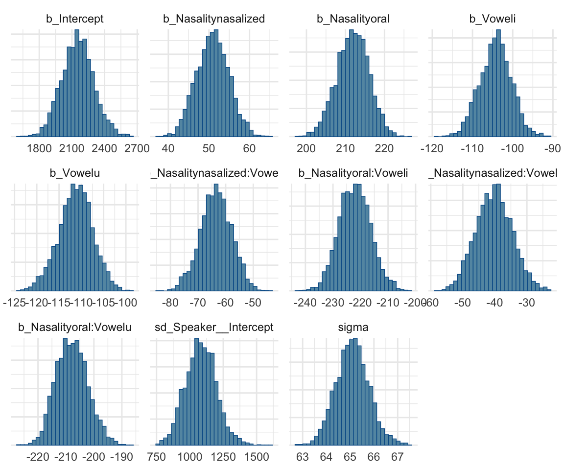

stanplot(f1modelcomplex, pars = c("^b","sd","sigma"), type="intervals")

## Warning: Method 'stanplot' is deprecated. Please use 'mcmc_plot' instead.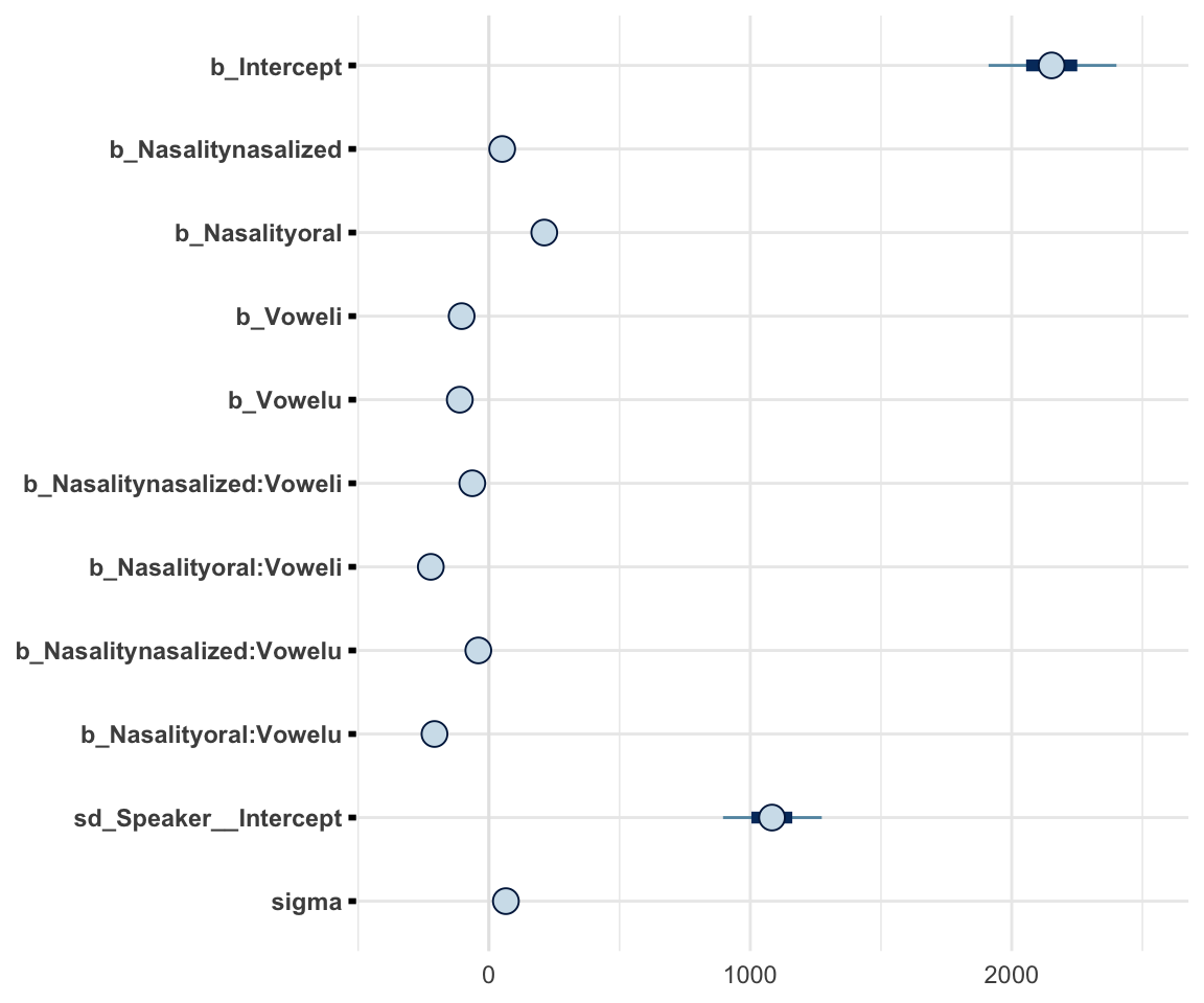

marginal_effects(f1modelcomplex)

## Warning: Method 'marginal_effects' is deprecated. Please use
## 'conditional_effects' instead.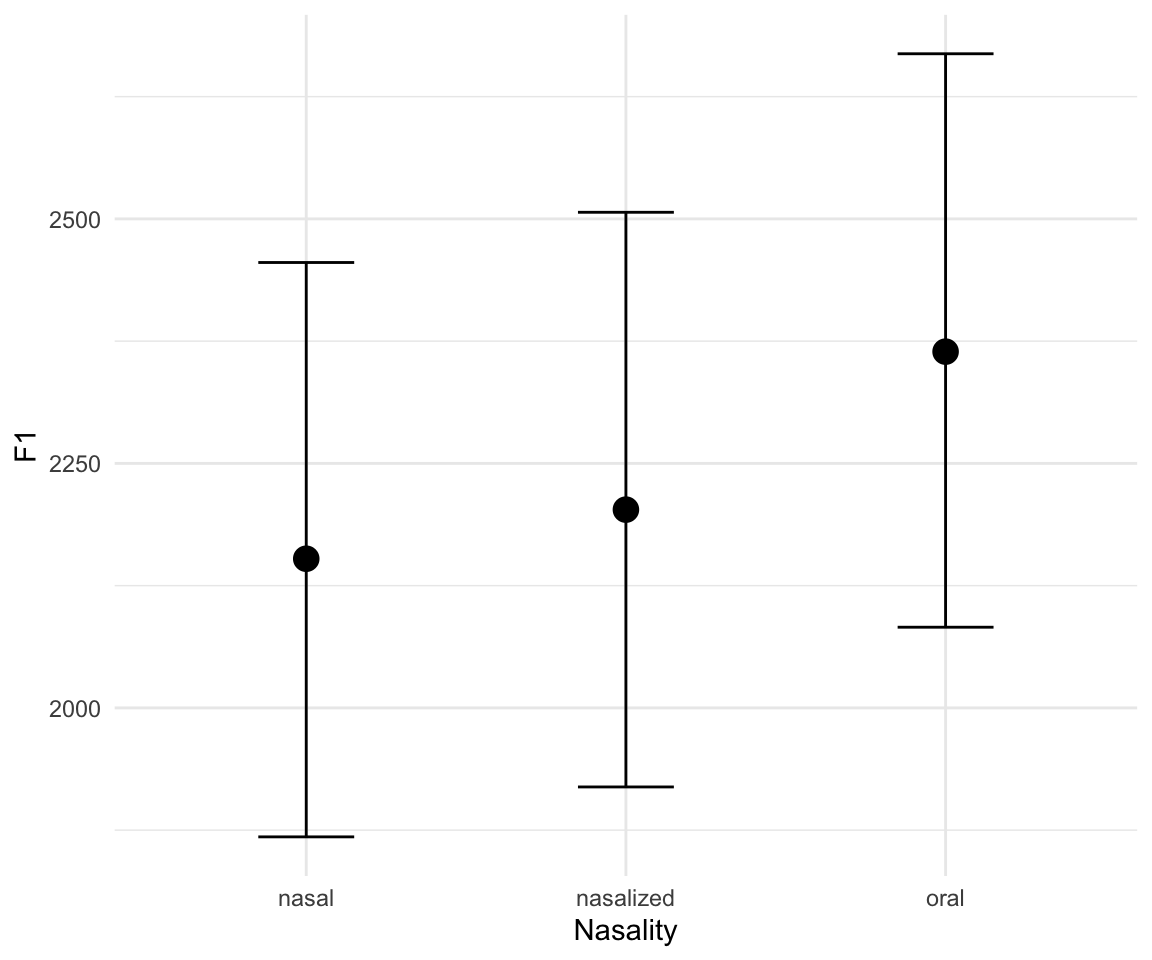

Note that there is a great interactive way to explore your models, using the shinystan package (though this cannot be run through HTML, so you will have to bear with me while I open it in my browser during class):

shinyml4 = launch_shinystan(f1modelcomplex)

Hypothesis testing

Hypothesis testing using CrIs

One way of doing hypothesis testing is to look at credible intervals: if the credible interval of a factor minus another factor crosses 0, it is unlikely that there are differences between those factors. We can do this in two ways: the first is taking the fitted values of the posterior for the data, and calculating the difference in the fitted values from the two factors. Since this will be a distribution, if the 95% CrI crosses 0, there is likely no difference, but if it doesn’t cross 0 there can be assumed to be a difference (with the difference being the mean).

f1modelcomplexfit= as.data.frame(fitted(f1modelcomplex, newdata = expand.grid(Vowel = levels(normtimeBP$Vowel), Nasality = levels(normtimeBP$Nasality)), re_formula = NA, summary = FALSE))

mylevels = expand.grid(Vowel = levels(normtimeBP$Vowel), Nasality = levels(normtimeBP$Nasality)) %>% mutate(PL = paste0(Vowel, Nasality))
colnames(f1modelcomplexfit) = mylevels$PL


head(f1modelcomplexfit)

##     anasal   inasal   unasal anasalized inasalized unasalized    aoral    ioral
## 1 1970.769 1862.541 1864.281   2025.140   1856.671   1872.579 2188.868 1860.258
## 2 2146.422 2043.369 2041.686   2195.662   2033.509   2048.600 2360.478 2039.744
## 3 2214.192 2111.770 2110.704   2262.647   2101.415   2118.879 2427.431 2106.283
## 4 2115.435 2007.839 2004.231   2169.349   1998.529   2011.101 2325.257 1994.175
## 5 2072.223 1963.479 1963.754   2121.961   1956.402   1972.644 2282.970 1954.022
## 6 1963.610 1856.974 1851.487   2012.519   1844.078   1861.560 2174.925 1852.669
##      uoral
## 1 1866.579
## 2 2043.784
## 3 2110.943
## 4 2001.746
## 5 1963.003
## 6 1852.065

f1modelcomplexfit = f1modelcomplexfit %>% mutate(anasoraldiff = (anasal - aoral), inasaldiff = inasal - (ioral + inasalized)/2, uioraldiff = uoral - ioral)
ggplot(f1modelcomplexfit, aes(x = anasoraldiff)) + geom_histogram()

## `stat_bin()` using `bins = 30`. Pick better value with `binwidth`.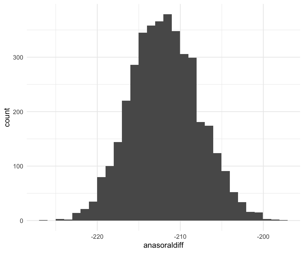

quantile(f1modelcomplexfit$anasoraldiff, c(0.5, 0.025, 0.975))

##       50%      2.5%     97.5% 
## -211.9408 -219.5889 -203.7939

ggplot(f1modelcomplexfit, aes(x = inasaldiff)) + geom_histogram()

## `stat_bin()` using `bins = 30`. Pick better value with `binwidth`.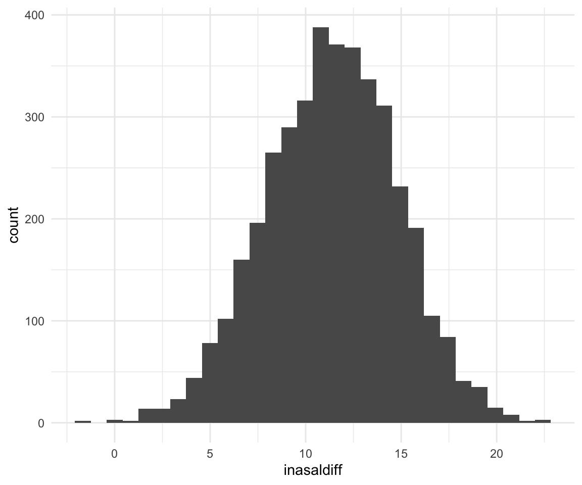

quantile(f1modelcomplexfit$inasaldiff, c(0.5, 0.025, 0.975))

##      50%     2.5%    97.5% 
## 11.42271  4.53596 17.96095

ggplot(f1modelcomplexfit, aes(x = uioraldiff)) + geom_histogram()

## `stat_bin()` using `bins = 30`. Pick better value with `binwidth`.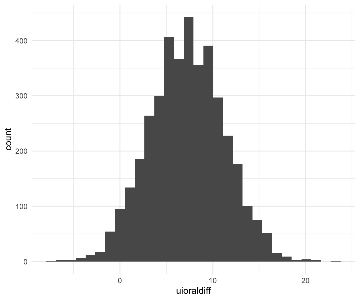

quantile(f1modelcomplexfit$uioraldiff, c(0.5, 0.025, 0.975))

##        50%       2.5%      97.5% 
##  7.2411039 -0.4768654 15.0091204

We can ask some research questions using the hypothesis function:

hypothesis(f1modelcomplex, "Intercept - Voweli = 0")

## Hypothesis Tests for class b:
##               Hypothesis Estimate Est.Error CI.Lower CI.Upper Evid.Ratio
## 1 (Intercept-Voweli) = 0  2257.67    148.17  1975.21  2559.32         NA
##   Post.Prob Star
## 1        NA    *
## ---
## 'CI': 90%-CI for one-sided and 95%-CI for two-sided hypotheses.
## '*': For one-sided hypotheses, the posterior probability exceeds 95%;
## for two-sided hypotheses, the value tested against lies outside the 95%-CI.
## Posterior probabilities of point hypotheses assume equal prior probabilities.

hypothesis(f1modelcomplex, "Intercept - Nasalitynasalized = 0")

## Hypothesis Tests for class b:
##                 Hypothesis Estimate Est.Error CI.Lower CI.Upper Evid.Ratio
## 1 (Intercept-Nasali... = 0  2102.48    147.93  1818.77  2404.06         NA
##   Post.Prob Star
## 1        NA    *
## ---
## 'CI': 90%-CI for one-sided and 95%-CI for two-sided hypotheses.
## '*': For one-sided hypotheses, the posterior probability exceeds 95%;
## for two-sided hypotheses, the value tested against lies outside the 95%-CI.
## Posterior probabilities of point hypotheses assume equal prior probabilities.

hypothesis(f1modelcomplex, "Intercept - Nasalityoral > 0")

## Hypothesis Tests for class b:
##                 Hypothesis Estimate Est.Error CI.Lower CI.Upper Evid.Ratio
## 1 (Intercept-Nasali... > 0  1941.54    148.05   1700.8  2188.85        Inf
##   Post.Prob Star
## 1         1    *
## ---
## 'CI': 90%-CI for one-sided and 95%-CI for two-sided hypotheses.
## '*': For one-sided hypotheses, the posterior probability exceeds 95%;
## for two-sided hypotheses, the value tested against lies outside the 95%-CI.
## Posterior probabilities of point hypotheses assume equal prior probabilities.

hypothesis(f1modelcomplex, "Voweli - Vowelu= 0")

## Hypothesis Tests for class b:
##            Hypothesis Estimate Est.Error CI.Lower CI.Upper Evid.Ratio Post.Prob
## 1 (Voweli-Vowelu) = 0     7.02      4.11    -1.19     14.9         NA        NA
##   Star
## 1     
## ---
## 'CI': 90%-CI for one-sided and 95%-CI for two-sided hypotheses.
## '*': For one-sided hypotheses, the posterior probability exceeds 95%;
## for two-sided hypotheses, the value tested against lies outside the 95%-CI.
## Posterior probabilities of point hypotheses assume equal prior probabilities.

Marissa Barlaz, PhD